More concentrated precipitation decreases terrestrial water storage

Data

TWS data come from the GRACE and GRACE-FO mass concentration solutions (RL06) developed by the Center for Space Research at the University of Texas²⁵. The dataset represents monthly total water mass variations (expressed as equivalent water height) at a gridded resolution of 0.25°. We omit data before August 2002 (due to sensor calibration at the outset of the GRACE mission) and for water-year 2017 (due to incomplete data during the mission gap between GRACE and GRACE-FO). We use GRACE TWS because it is an observational data product that holistically measures land water, capturing all surface and underground stocks.

To account for observational uncertainty, we use three daily gridded precipitation data products: the Global Precipitation Climatology Project (GPCP) Daily Precipitation Analysis v.1.3 (ref. ²¹), the Global Precipitation Climatology Center (GPCC) Daily Analysis v.2022 (ref. ²³) and the National Oceanic and Atmospheric Administration Climate Prediction Center (CPC) Unified Gauge-Based Analysis²². GPCC is a station-based product (1° resolution) with coverage over 1982–2020, whereas CPC (0.5°) and GPCP (1°) integrate station and satellite observations over 1979–2022 and 1997–2022, respectively. We repeated our analysis for the more recent GPCP v.3.3 and find consistent main effects⁵⁶ (Supplementary Fig. 4), but use the more complete earlier version for our main analysis (GPCP v.3.3 contains missing daily values at high latitudes after 2020).

We use two net all-sky surface shortwave radiation datasets: the Global Energy and Water Exchanges Surface Radiation Budget (GEWEX-SRB, limited here to 2002–2017)⁵² daily dataset and the NASA Clouds and the Earth’s Radiant Energy System Energy Balanced and Filled monthly dataset (NASA-EBAF, limited here to 2002–2022)⁵³, each at 1° resolution. We use monthly evapotranspiration from the GLEAM v.3.8a, at 0.25° resolution for the overlapping GRACE period (2002–2020; ref. ⁵⁴). Main river basin boundaries are from the HydroBASINS v.1.0 dataset, which is derived from Shuttle Radar Topography Mission elevation data collected in 2000 (ref. ⁵¹). All data URLs are enumerated in Supplementary Table 1.

Daily climate model data are from the land-hist experiment of the Coupled Model Intercomparison Project, Phase 6, Land-Surface, Snow and Soil Moisture Intercomparison Project (CMIP6-LS3MIP)⁵⁵. In the land-hist experiment, the land-surface components of climate models are forced by atmospheric forcings from the Global Soil Wetness Project phase 3, whose precipitation data are derived from the NOAA-CIRES-DOE Twentieth Century Reanalysis (20CR). We include results from the two models that report all required variables: MIROC6 with land component MATSIRO and VISIT-e⁵⁷, and CNRM-CM6-1 with land component ISBA-CTRIP⁵⁸. We use the mrtws (total water storage), tas (mean surface air temperature) and pr (precipitation rate) variables. No participating models report these required variables plus evaporation, precluding extending our climate model analysis towards mechanisms.

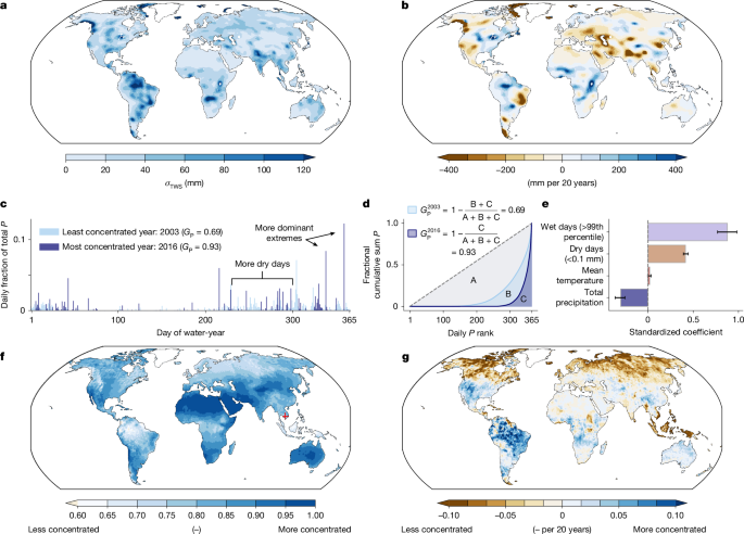
Data aggregation and precipitation Gini coefficient

All data are temporally aggregated to the water-year scale, using October to September for the Northern Hemisphere water-year and July to June in the Southern Hemisphere. On this water-year scale, snow and ice storage changes are negligible. We further limit our spatial domain to regions without permanent snow and ice accumulation. We compute daily mean temperature data using the average of daily maximum and minimum temperatures from CPC. We also compute climatological mean precipitation as the average of the annual total over the full precipitation data record.

We linearly detrend GRACE data to isolate interannual variability, which is largely governed by hydroclimate variability, from long-term trends that include anthropogenic water use and management^26,31. The rationale for this focus on interannual variability is to establish whether more concentrated daily precipitation distributions lead to cumulative water balance changes, averaged across the water-year, absent the influence of coincident economic, demographic and mean warming trends.

Correspondingly, and because GRACE only estimates TWS relative anomalies, we detrend and demean all other hydroclimate variables (except climatological precipitation, which is time-invariant). Finally, we interpolate all datasets to a common 0.5° grid as a compromise across the resolutions of the datasets. We repeated our analyses at alternative coarser common resolutions (1°, 2° and 3°) and found consistent results (Supplementary Fig. 5). We present long-term linear trends in terms of changes per 20 years to ease interpretation.

To quantify the annual concentration of daily precipitation, we apply the Gini coefficient, a common economic measure of income inequality⁵⁹, to the three daily precipitation datasets. The Gini coefficient is based on the Lorenz curve, which plots the cumulative share of the total quantity (that is, cumulative share of annual precipitation) against the cumulative share of the population (that is, days per year), sorted from least to greatest (Fig. 1d). The Gini coefficient is defined as the area between the Lorenz curve and the 1:1 line of equality. For more concentrated distributions, such as all of the annual precipitation falling in 1 day, the Lorenz curve deviates further from the line of equality, giving a Gini coefficient closer to 1. If all days are equally rainy, the Gini yields a value of 0. We use a computationally efficient discrete formulation to calculate the annual Gini coefficient of sorted daily precipitation (G_P):

where n is the number of days per year and P is a sorted vector of precipitation values for a given water-year and location. The cumulative sum of P approximates the Lorenz curve (inner numerator double summation), and the normalized integral of that curve is estimated by summing the cumulative values (outer numerator double summation) and dividing by the total sum (denominator summation). This formulation is analytically identical to more common Gini formulations, but is computationally faster. As with the other variables, we linearly detrend and demean G_P to isolate local interannual anomalies.

G_P is—by formulation—sensitive to both incremental dry days and precipitation extremes. These joint sensitivities are mathematically coupled: in normalized terms, incremental dry days necessitate a greater concentration of annual precipitation into the remaining wet days, whereas incremental precipitation extremes leave less annual precipitation to be distributed across the remaining days of the year. This coupling maps conceptually with expectations from the physics of hydrologic intensification, in which daily precipitation responds more to warming than its annual total. We confirm this joint sensitivity of G_P by regressing its annual anomalies on annual occurrence of extreme precipitation days (>99th percentile of nonzero precipitation days), dry days (<0.1 mm), and total annual precipitation as well as on annual mean temperature.

Statistical models of TWS effect

For each precipitation dataset, the data aggregation and G_P calculations yield a panel of annual anomalies in TWS, mean temperature (T), total precipitation (P) and G_P, plus long-term (absolute) climatological mean precipitation (\(\bar{P}\)). The three panels vary in sample size because of differing time availability of the precipitation datasets (Supplementary Table 2).

To assess the influence of G_P on TWS for each panel, we apply linear fixed-effects models, a type of panel regression that enables controlling for time-invariant unobserved spatial heterogeneity using spatial fixed effects, as well as global shocks in any year using time fixed effects⁶⁰. Our approach minimizes confounding by spatial or temporal trends in environmental, climate or anthropogenic factors that may covary with G_P, without explicit inclusion in the model. Spatial fixed effects remove all static differences across grid cells, such as baseline differences in soils, hydrogeology, vegetation and groundwater use or irrigation infrastructure. Water-year fixed effects absorb global shocks that affect all regions simultaneously (notably, El Niño events). By detrending all variables, we also exclude long-term groundwater depletion trends, ensuring that the model captures only interannual variability.

This identification strategy isolates the emergent interannual influence of precipitation concentration on TWS. The models are of the form

where θ and π are coefficients of temperature and annual precipitation, σ and τ are spatial and time fixed effects, superscripts i and t denote grid cell and water-year, and ε is the residual. These terms are included as controls for the influence of other hydroclimate or unobserved variables. We estimate the effect of G_P as an interaction with climatological mean precipitation (using linear coefficient γ and interaction coefficient χ) to explicitly assess variation in the effect across the global aridity gradient. As such, the marginal effect of an anomaly ΔG_P on TWS is conditional on climatological precipitation and is given by

We interpret this marginal effect as the generalizable response of local interannual TWS variation to local anomalies of precipitation concentration, conditioned on local climatological wetness. We present the marginal effect of G_P on TWS per a 10 percentage-point change in G_P (that is, a G_P anomaly of 0.1) as G_P values are bounded between 0 and 1, and vary interannually by a smaller portion of that range. For each precipitation dataset, we estimate the coefficients in equation (2) separately using absolute anomalies (to quantify the effect in hydrologically meaningful units) and standardized anomalies (to enable comparison of effect sizes across predictors). Coefficients are estimated using the lfe package in R. Global Pearson correlation among predictors (pooled across space and time) is under 0.5 (r² under 0.25), indicating little scope for influence of collinearity on regression estimates (Extended Data Fig. 10). To ease visualization of standardized coefficients, we present the conditional G_P effect at the global population-weighted climatological mean precipitation value of 1,000 mm.

As the marginal effect of G_P on TWS is conditioned on climatological precipitation, its standard error depends on the variance of coefficients χ and γ as well as the climatological precipitation. We estimate this standard error (SE) using the variance of linear combinations of estimators:

When estimating the variances and covariance of χ and γ, we cluster standard errors at the main river basin scale to account for spatial and temporal autocorrelation of gridded data⁵¹—this step yields more conservative standard errors and avoids type-I errors due to the non-independence of observations. We also tested Conley spatial standard errors⁶¹ with distance cutoffs of 300 km (roughly the effective resolution of GRACE) and 750 km (the average length scale of global river basins in HydroSHEDS; Supplementary Fig. 6a–c), and Driscoll–Kraay temporal standard errors with time cutoffs of 3 years and 5 years (Supplementary Fig. 6d–f). All approaches yield similar confidence intervals. At a given value of climatological precipitation, we consider the marginal effect of G_P on TWS as statistically significant, for which its median estimate plus or minus two standard errors excludes zero.

We also estimate a reduced form of equation (2) at the main river basin scale to check the robustness of the global effect at finer spatial scales⁵¹, and to characterize its spatial variability. We omit the interaction between G_P and climatological precipitation, as variation in climatological precipitation within basins is smaller than across the globe. For simplicity, we present these basin-scale TWS effects as the average across the three products, wherever they are significant (P < 0.05) and of consistent sign in at least two of the three precipitation data products. Basin-scale TWS effects are fairly consistent across the three data products (Extended Data Fig. 5).

Although spatial fixed effects control for time-invariant spatial differences, they do not control for confounders that vary interannually in response to G_P itself, such as irrigation responses to year-to-year variation in TWS change, which might deplete groundwater. To isolate the influence of irrigation, we add an interaction term, I, for the grid cell area equipped for irrigation to equation (2) (using data from the UN Food and Agriculture AQUASTAT Global Information System on Water and Agriculture):

In this model, the influence of G_P on TWS depends on both climatological mean precipitation and irrigation area, which we evaluate at varying levels. The approach enables our isolation of irrigation influence, despite 95% of grid cells in our analysis containing <1% irrigated area.

For the CMIP6-LS3MIP land-hist climate model data, we apply the identical data aggregation and statistical modelling in equations (2–4) to the simulated TWS, T, P and G_P. To test the robustness of the estimated TWS effect to temporal and spatial variability in gauge coverage, we regress the basin-level TWS effects on the on basin mean areal gauge density (gauges per basin) and on the coefficient of variation of the number of gauges per basin over time (standard deviation of gauges per basin divided by the average), based on the GPCC gauge count data. The relationships show no significant dependence of the basin-level TWS effect on areal station density or the degree of year-to-year variation in gauge density (Extended Data Fig. 6b,c). Empirical results using only GRACE (through water 2016) and excluding GRACE-FO (2018–2022) are consistent with those using the complete GRACE record⁶² (Supplementary Table 3).

Statistical models of effect mechanism

To clarify the mechanism of the effect of G_P on TWS, we develop two companion panel regressions similar to those used to assess the TWS effect, but using GLEAM evapotranspiration (E) and shortwave radiation (S) anomalies from GEWEX-SRB and NASA EBAF in place of TWS in equation (2). To isolate the intensity-partitioning mechanism of the TWS effect, we add a regressor in the form of shortwave radiation anomalies in equation (2) to explicitly control for the radiative effect of additional dry days:

We model the effect of S on TWS, including an interaction with climatological precipitation to account for variable effects across gradients of mean aridity (and thus energy compared with moisture limitation). As such, ζ is the TWS sensitivity to shortwave radiation anomalies and ψ is the interaction effect with mean precipitation. The prime symbols indicate coefficients estimated with the S control, to distinguish from coefficients in equation (2).

Introducing the S control removes the TWS variance attributable to shortwave anomalies, which are positively correlated with G_P, from the estimated G_P effect. We consider this positive S–G_P correlation as a facet of the hydrologic effects of precipitation concentration, so we omit this control when estimating the full TWS effect. However, we include the S control in equation (6) to isolate the land-surface hydrologic partitioning effects of daily precipitation distribution on TWS, apart from the fact that more concentrated precipitation years are sunnier. We interpret this isolated effect as the influence of more intense precipitation on surface partitioning, such as infiltration-excess or saturation-excess ponding of precipitation on the surface.

For simplicity, we present this partitioning effect as an average of effects across the three precipitation datasets, with uncertainty characterized as the maximum and minimum of the full two standard error interval across the three precipitation and two radiation data products. This approach is conservative, as standard errors would be smaller if we first averaged the precipitation data, rather than averaging effects. However, results for individual datasets are consistent with those from the three-product average (Supplementary Fig. 1). To estimate the relative fractional contribution of the partitioning effect to the full effect (f_D), we divide the partitioning effect by the marginal effect estimated using equations (2) and (3):

Because it is simpler to visualize, we present this fractional distribution effect both for the average across data products and for each individual product (based on the data in Supplementary Fig. 1).

Reanalysis models contain appreciable biases in the simulation of daily precipitation, especially for extreme values that contribute disproportionately to annual precipitation and strongly influence concentration⁶³. As such, we favour an empirical approach based on observational hydroclimate and TWS data. But understanding the mechanism of the observed effect requires assessing surface water budget terms that are poorly observed globally. We use GLEAM evapotranspiration data to establish the plausibility of evapotranspiration responses to G_P. But as GLEAM assimilates precipitation data (and thus biases) from reanalysis, it probably underrepresents daily precipitation concentration effects. We similarly use the FLUXCOM CERES-GPCP flux-tower based energy and water flux dataset (2001–2014) to provide an in situ window on evaporative responses to precipitation concentration⁶⁴; however, as its observational constraint is limited to the approximately 100 m radius surrounding the tower, these data are not comparable to GLEAM, estimated on a 0.25° grid. To overcome these observational limitations on water-budget terms (evaporation and runoff), we extend a simple, process-based land–atmosphere model with hydrology⁶⁵, driven by the daily precipitation datasets at a set of grid points sampling the global precipitation gradient.

Idealized land-surface model

We use an idealized process-based land-surface model to provide additional evidence for the negative TWS effect of G_P and to clarify its mechanism (the underlying surface water balance changes and their drivers). Although more complex land-surface contain more complete process representations, the ultimate energy–moisture balance rests on nested and coupled parameterizations, making a mechanistic diagnosis difficult, if not impossible.

Embracing recent community calls for robust and simple theories of land surface climate¹¹, we run land-surface model simulations that parsimoniously capture variations in surface precipitation partitioning and land–atmosphere coupling. We use experimental design that enables direct comparison with the observed TWS effect. First, as the observed TWS effect is due to G_P anomalies and because GRACE TWS measures anomalies, we focus on simulating the sensitivity of TWS to changes in G_P, rather than mean TWS itself. Second, our statistical model includes space fixed effects to capture time-invariant differences in land cover and soil characteristics. Our idealized model mirrors this approach by using median parameters globally, rather than calibrating parameters locally. In short, rather than developing and validating a complete and realistic model of all of the processes driving TWS, we develop the minimal physics required to plausibly explain our observational results and assess the most important underlying processes.

Our process-based model parsimoniously represents the coupled surface partitioning of precipitation and energy–moisture balance. It extends the one-dimensional simple energy–moisture balance (SEMB) model, developed in ref. ⁶⁵, to represent precipitation partitioning at the land surface and simulate a surface water stock (Extended Data Figs. 9 and 10). In the original model formulation, precipitation infiltrated instantaneously into the soil moisture stock (M_S), irrespective of its intensity. On saturation, excess runoff was treated as an instantaneous water flux outside the model domain, precluding evaporation from surface water within the model. Our extended model (SEMB with hydrology, SEMB-H) includes intensity-dependent surface partitioning of precipitation towards infiltration compared with infiltration and saturation excess, the latter two being retained within the model using a surface water stock (M_L), whose outputs include evaporation and runoff. Physically, these developments allow the model to more completely represent surface precipitation partitioning processes: when precipitation meets the land, water can pool at the surface if the infiltration capacity of the soil or maximum saturation have been reached, and this ponded surface water can run off or evaporate.

The surface energy balance is given in terms of time-evolving surface air temperature (T) as

where C is the effective heat capacity of the soil layer, F_SW is the net surface shortwave radiation, D is the sum of net longwave radiation and the ground and sensible heat fluxes (that is, the ‘dry’ energetic response), E_S is evaporation from soils and L is the enthalpy of vapourization of water. Following ref. ⁶⁵, D is parameterized as a function of the dewpoint depression (\(T-\bar{{T}_{{\rm{D}}}}\)) using a dry energetic parameter α, representing the temperature-damping efficiency of non-evaporative fluxes. We derive the value of α from ref. ⁶⁵, estimated by regressing the sum of longwave, sensible heat and ground heat fluxes on the surface dewpoint depression temperature in ERA-Interim reanalysis. Evaporation is parameterized as a function of vapour pressure deficit (\({q}_{\mathrm{sat}}(T)-\bar{q}\)) by r_S, which is the bulk soil surface resistance (ρ_a is the mean density of air). Atmospheric humidity variables (\(\bar{q}\) and \(\bar{{T}_{{\rm{D}}}}\)) are fixed to climatological mean values, as local variability in atmospheric evaporative demand is more strongly related to temperature than specific humidity variation. Evaporation is also a linear function M_S (that is, soil wetness), expressed in terms of saturation state.

The change in soil moisture stock is precipitation less soil evaporation, infiltration and saturation-excess ponding rate of water, and soil drainage. We simulate it as

where P is daily precipitation, Q_S is ponded surface water (infiltration excess and surface excess), Q_D is soil drainage (also known as subsurface runoff in many land-surface models) and μ_S is a geometric parameter to convert between water equivalent heights and saturation state. Q_S is parameterized using the US Soil Conservation Service Curve Number scheme developed by the United States Department of Agriculture^66,67,68, which posits a quadratic increase in the surface ponding rate (saturation and infiltration excess) as a function of daily precipitation intensity and a parameter, S, that captures the maximal retention of soil water:

In this parametrization, λ is a parameter representing the ratio between initial abstraction of precipitation and potential maximum soil water retention (S), which determines the minimum daily precipitation at which ponding occurs. Beyond this minimum, surface ponding rate increases according to the curve number (CN) parameter (a value between 0 and 100), which reflects the surface ponding rate sensitivity to precipitation intensity. We use CN values of 30 (dense forest cover), 50 (sparse woody vegetation on sandy loam soil) and 80 (grassland or impervious surfaces) in our model experiments⁶⁷. The soil drainage (or subsurface runoff term), Q_D, is parametrized in terms of unsaturated hydraulic conductivity:

where k_sat is the saturated hydraulic conductivity and c is parameter controlling the nonlinear response of soil water leakage to soil saturation states above the field capacity⁶⁹. Parameter values are for median sandy loam soils (Supplementary Table 3).

A key innovation in the model is to assess the potential for precipitation to pool on the land surface and evaporate before it contributes to total runoff. We model ponded surface water and soil drainage as contributing to the surface water stock (M_L), which is governed by

where E_L is evaporation form the surface water stock, Q_L is runoff out of the surface water stock, and μ_L is a geometric parameter to convert between water equivalent heights and saturation state (that is, fractional ‘fullness’ of the reservoir). In our specification, Q_D, or soil drainage, contributes to surface water stocks, reflecting the dominant contribution of soil drainage to streamflow through subsurface flow^70,71. E_L is parametrized similarly to E_S, but as a function of M_L instead of M_S and with a lower bulk surface resistance (r_L). This lower resistance captures stomatal control on transpiration over land, and the fact that water evaporates more easily from a free surface (Supplementary Table 3). As our model stipulates a minority areal fraction covered by the surface water stock (10% in the median parameters; Supplementary Table 3), we assume that the temperature (and thus vapour pressure deficit) over surface water is dictated by the energy balance over soils. This simplification enables us to simulate E_L without simulating horizontal transfers within the atmosphere, but results are similar using a simple bulk temperature-homogenization scheme (Supplementary Fig. 7). Q_L is parametrized as a quadratic function of M_L and a maximum fractional daily outflow rate parameter (ω), such that Q_L = ωM_L². In this formulation, runoff occurs only at the boundary of the model, enabling the model to track whether ponded surface water evaporates before leaving the grid cell. We use a global mean range of ω values based on the mean turnover rate of freshwater in lakes and reservoirs, estimated as the ratio of mean runoff (5 × 10⁴ km³ yr⁻¹; ref. ⁷²) to global total surface freshwater volume (2 × 10⁵ km³; ref. ⁷³), or around 0.1% per day. We also run the model with larger ω values (0.5–1% per day) to account for the volumetric dominance of large, slowly overturning lakes.

We initialize our model at a surface air temperature of 280 K and with a saturation state of 0.5 for the soil and surface water stocks. In contrast to more complex land-surface models featuring deep soil water stocks, all prognostic variables are governed by fast first-order dynamics with characteristic e-folding times of the order of days, as defined by the geometry, parameters and forcings of the model. As such, we run our idealized model experiments without a multi-year spin-up common for complex land-surface models.

Land-surface model experimental design

To simulate the TWS effect using SEMB-H, we run the model using P and F_SW forcings from CPC and GEWEX-SRB at 1,400 points randomly sampled across the global range of climatological precipitation. At each location, we run the model twice, using forcings for the highest and lowest G_P year available in the observational CPC data. This approach captures variation in both daily P and S and how they, in turn, shape G_P. To isolate the effect of G_P from that of annual precipitation, we scale the daily P time series from each of these two years to ensure that they have equal totals (Extended Data Fig. 8). This eliminates confounding TWS effects of low and high precipitation years, analogously to our control for annual precipitation in equation (2). We estimate the simulated TWS effect (ΔTWS_sim) as the difference between maximum and minimum G_P years in volume-weighted sums of M_L and M_S. To match the water-year scale of our empirical analysis, we take this difference as an average across the water-year (denoted by overbars):

where a_S and a_L are the areal fractions of soil compared with surface water stocks. As these simulated TWS responses reflect a wide range of actual G_P differences, we linearly scale ΔTWS_sim to a uniform 0.1ΔG_P as in our empirical analysis. Finally, we express the simulated TWS effect as a global statistical relationship in terms of climatological precipitation, for comparison to our empirical results:

where i denotes points in our sample. As we keep annual precipitation and surface parameters constant in our simulations, equation (15) is analogous to equation (2), such that β₀ and β₁ are the simulated equivalents of γ and χ. We estimate uncertainty in equation (15) analogously to in equation (4), and compare the confidence intervals of the empirical and simulated TWS effects. We also track the mean differences in water-year totals of E_L, E_S, Q_S and Q_L between the maximum and minimum G_P years to attribute the TWS effect to surface water budget changes. E_L reflects evaporation from ponded surface water as well as from initial moisture stocks, as E_L is initialized at 0.5 (that is, half full), and as such is not necessarily limited by Q_S.

The main free parameters in SEMB-H are the dry radiative coefficient (α), the CN, the fractional daily outflow rate from the surface water stock (ω) and the geometric parameters governing the potential height and fractional area of the soil and surface water stocks (h and a). To test the robustness of our simulation results to values of these free parameters, we rerun the simulations using 243 combinatoric parameter sets at the 1,400 points (a total of about 365,000 simulations; Supplementary Table 3), and compare the range of simulated TWS effects (equation (15)) to the confidence intervals of the empirical effect. We further characterize the relative influence of free parameter values on the simulated TWS effect using Sobol’s indices, a variance-based sensitivity analysis across the full parameter space⁷⁴. This analysis allows us to assess how uncertainty in each parameter, individually and jointly (through interactions), affects uncertainty in the simulated TWS effect.

Imputed TWS changes

Using the global coefficients from equation (2) and local climatological precipitation across global land area, we estimate the TWS impact of G_P trends (\(\Delta {\mathrm{TWS}}_{\mathrm{hist}}\)) over 1980–2022 using

In this formulation, TWS impacts depend on climatological precipitation and concentration trends at a given grid cell (superscripts i). This approach assumes that TWS effects of concentration, as estimated from detrended interannual variability, operate similarly over multi-decadal trends. We present the imputed historical TWS impact as an average across data products for simplicity.

To project future TWS impacts of concentration under continued global warming, we first use a simple thermodynamic model to project daily precipitation distribution changes under mean warming across global land⁴⁵. This model enables efficient and transparent estimates of future concentration globally, isolated from the influence of long-term annual precipitation changes and avoids consistent daily precipitation biases in general circulation models. The model intensifies observed daily precipitation distributions (I) at a fractional scaling rate of φ per degree of local warming (ΔT):

For φ, we use the Clausius–Clapeyron saturation vapour pressure sensitivity to temperature of 7% °C⁻¹, drawing from observational literature linking daily precipitation intensity to temperature^8,75. Our goal is to briefly contextualize the TWS implications of median concentration expectations, so here we do not explore uncertainty in this parameter. For the initial observed intensity, I, we use daily precipitation distributions for the water-year with G_P closest to the long-term median. Precipitation intensification is projected at an illustrative 1 °C of global mean surface air temperature warming beyond the study period (or about 2 °C above the pre-industrial limit), in line with current plausible mitigation scenarios for the late-twenty-first century. The local surface air temperature warming pattern at 1 °C of global mean warming is derived from the average of 26 CMIP6 models⁷⁶, run under the SSP5-8.5 scenario.

Annual precipitation generally changes by less than 7% °C⁻¹, implying an increase in dry days. Consistent with our empirical model formulation, we enforce constant annual precipitation to isolate the influence of concentration changes under warming. To achieve this, we offset the increased precipitation from intensification by converting the lowest-M precipitation days to dry days, where M is the number of days for which the total precipitation equals the intensification-induced annual increase. We then difference the G_P of this final concentrated distribution from the G_P of the initial, observed distribution to estimate G_P changes under warming. These projected G_P changes are of similar order to historical trends (1–10 basis points; Fig. 1g and Extended Data Fig. 3).

Finally, we use this G_P-change field to project changes in TWS, as in equation (16). Apart from mapping local TWS impacts, we also estimate global population exposure to standardized mean TWS changes using population data from the Intersectoral Impact Model Intercomparison Project⁷⁷. We first project the TWS impacts onto the population data to derive a frequency distribution of exposure, then quantify the proportion of the global population experiencing standardized anomalies exceeding 0.5 standard deviations—an illustrative threshold indicative of abnormally dry conditions¹⁰. We simply provide a median estimate for these population exposure estimates as a first-order characterization the global importance of these effects. Importantly, our approach assumes that spatial and temporal patterns of global irrigation remain constant in the future. Because intensively irrigated areas experience a stronger TWS effect from precipitation concentration (Extended Data Fig. 6a), expansion or intensification of irrigated areas could lead to locally stronger future drying. Conversely, improvements in irrigation efficiency may reduce withdrawals per unit area in response to precipitation concentration.