An X-linked long non-coding RNA, PTCHD1-AS, and the core features of autism

Phenotype–genotype analysis

Ethics statement

This research involving human participants complies with all relevant ethical regulations, including obtaining informed consent from all participants through the recruitment sites. Ethical review and approval were obtained from The Hospital for Sick Children Research Ethics Board (REB 1000080561).

ASD-associated genetic variants at the PTCHD1-PTCHD1-AS locus in ASD cohorts

We analysed MSSNG, Simons Simplex Cohort and SPARK ASD WGS databases for genomic variants at the PTCHD1-PTCHD1-AS locus, with ethics approval and informed consent for the MSSNG database as previously described^4,51. MSSNG cohorts contain family data with at least one child having a diagnosis of ASD. Rare microdeletion variants are defined as those less than 1 Mb in size and occur at a frequency of below 1% in control population cohorts. Variants meeting these criteria are then evaluated for ASD risk, and corresponding phenotype data are collected.

Frequency impact of rare deletions across the PTCHD1-PTCHD1-AS locus

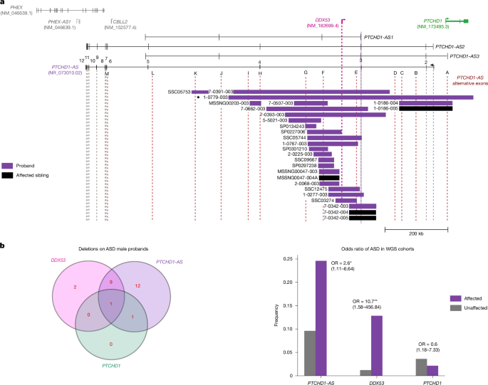
We conducted a comparative analysis of the frequency of rare copy-number deletions (populational frequency less than 1%) overlapping the target exons on PTCHD1-AS, as well as PTCHD1 and DDX53. We assessed deletions with a length of 1 kb or more, identified as previously described⁵² across three independent ASD cohorts (MSSNG, SSC, and SPARK)^4,15,53, contrasting with six independent control cohorts (1000 Genomes Project, 1,234 male individuals⁵⁴; MGRB, 1,756 male individuals^55,56; HostSeq, 4,235 male individuals⁵⁷; CHILD, 203 male individuals⁵⁸; INOVA, 100 male individuals, www.inova.org); cardiomyopathy⁵⁹ and congenital heart disease cohorts, 804 male individuals⁶⁰). Our analysis exclusively considered high-quality deletions, meeting the following criteria: (1) length of at least 1 kb; (2) identification by both ERDS⁶¹ and CNVnator⁶², with at least 50% reciprocal overlap between the two methods; (3) less than 70% overlap with repetitive or low complexity genomic regions (such as telomeres, centromeres and segmental duplications); (4) exclusion of CNVs in the pseudoautosomal regions or X chromosomal calls in males. We then used Fisher’s exact tests to compare the occurrence of overlapping deletions in male individuals within each target region between probands and control cohorts, resulting in final P values and ORs. The final comparison includes all PTCHD1-AS from exons 2 to 5, including the novel exons. We also analysed deletions overlapping DDX53 and PTCHD1 for comparison purposes.

Analysis of genotype–phenotype relationship in NDD cohorts at the PTCHD1-PTCHD1-AS locus

In ASD-specific cohorts with WGS data or any technology and primary diagnosis of ASD, individual data from the publicly available database DECIPHER v.11.27 and Lineagen (a private genetic diagnostic company) were accessed in September 2024 and February 2017, respectively. The individual selection and cohort descriptions are summarized in Supplementary Table 18. Here the primary diagnosis is the main NDD. Secondary diagnoses may include other disorders (such as ADHD, ADD, obsessive–compulsive disorder), other neurological conditions (epilepsy, presence of seizures) or additional mental health conditions (anxiety). Records of each database were obtained first by searching for PTCHD1-AS or PTCHD1 loss of function genetic variants in all databases or published cohorts.

Mouse models

We used Benchling (http://benchling.com/) to design guide RNAs and excised mouse Ptchd1-as (Gm15155-201) exon 3 (237 bp) and 150 bp on either side, generating two mutant mice both containing a patient-like deletion of exon 3: (1) Ptchd1-as^−Ex3 (KO-1); and (2) with an insertion of 168 bp intronic tandem poly(A) sequence⁶³ within the lncRNA transcript, termed Ptchd1-as^−Ex3-is (KO-2). Guide RNAs (5′-AGGTTAGCATTATACCACTG-3′ and 5′-GTCTCCACATTTACATACTC-3′) on each side of Ptchd1-as exon 3 were used to create double-stranded breaks and KO-1 mice. A single-stranded intronic oligonucleotide (TCATGATGTTTTGTCCAGGAATAGAAACCCTGACTAAGATACTAGGTTAGCATTATACCAAAATAAAATACGAAATGTGACAGAAAATAAAATACGAAATGTGACAGACTCAGGTTTGTCTACTTTTCTTCATGTTTTAGGAATACGAGACTTATGGACACCAATAAT), including the tandem copies of the neuropilin-1 poly-adenylation sequence (bold), was included with guide RNAs and Cas9 in the injection mix to generate KO-2 mice.

CRISPR–Cas9 editing was performed at the Centre for Phenogenomics as previously described⁶⁴. Founder mice were backcrossed 3–5 generations onto strain C57BL/6J and to refresh the line every third generation. KO-1 and KO-2 mice were validated by PCR break-point analysis. Off-target analysis was performed by WGS and comparison to the C57BL6/J reference sequence using Mutect2 (GATK3.7). No exonic mutations were detected in the initial backcrossed line for either strain.

The primers for genotyping (forward, 5′-GAACAGTGGTTTGGAGGTGTAA-3′; reverse, 5′-TGTTCTGTGAGTTGGGCATATC-3′) detect a single band at 364 bp for KO-2 and at 314 bp for KO-1 mice, representing hemizygous males. WT male mice have a 553 bp fragment.

Mouse management conditions

KO-1 and KO-2 (male hemizygous; C57Bl/6J) mice and their WT littermate mice were used for all behaviour experiments. The mice were bred at the Hospital for Sick Children or The Centre for Phenogenomics, Neurobehavior Core and group-housed in cages with 3–5 mice per cage. The housing conditions maintained a constant temperature of 22 °C and a 12 h–12 h light–dark cycle, with food and water available ad libitum. All of the procedures were approved by the Hospital for Sick Children Animal Care and Use Committee (AUP 49151) and The Centre for Phenogenomics Animal Care and Use Committee (AUP 25-0307; 20-0307H) and conducted in accordance with Canadian Council on Animal Care guidelines. Electrophysiological recordings were carried out at the Lunenfeld Tanenbaum Research Institute in Mount Sinai Hospital, Toronto (AUP 24-0292H) and at the University of Toronto’s, Tanz Centre for Research in Neurodegenerative Diseases, University Hospital Network (AUP 6668.8). Mice were bred and group-housed under similar conditions as described above. Tissues samples for electrophysiology, ddPCR, RNA-seq and proteomics were obtained mainly from mice housed at the TCP unless otherwise stated. Age-matched mice between 8 and 12 weeks of age were used for testing in 2 to 3 different behaviour tests. All of the experiments took place during the light phase and were conducted and analysed in a blinded manner, with the experimenter unaware of the experimental conditions. The sample sizes were determined on the basis of established standards in the field and previous experience with phenotype comparisons. No statistical methods were used to predetermine the sample size.

MRI brain imaging

In total, 50 mice were used for the brain imaging experiments (23 hemizygous male mutants and 27 WT littermate male controls). Each mouse was scanned repeatedly from the early post-natal period into young adulthood according to methods and procedures described previously⁶⁵. The precise time of scans was jittered for each mouse, and not all mice were continued into adulthood.

Image acquisition

Twenty-four hours before each scan, a 0.4 mmol kg⁻¹ dose of 30 mM manganese chloride (MnCl₂) was administered as a contrast agent. For mice that were 10 days old or younger, the dam was intraperitoneally injected with MnCl₂, and pups received MnCl₂ through maternal milk. Mice that were over 10 days of age received intraperitoneal injections of MnCl₂. Up to four mice were scanned simultaneously. Custom-built 3D-printed holders, which allowed anaesthetic delivery and scavenging, and heating were used. During the scan, mice were anaesthetized with 1–2% isoflurane, and the respiratory rate was monitored using a self-gated signal from a modified 3D gradient echo sequence⁶⁶.

A multi-channel 7.0 T MRI scanner with a 30 cm diameter bore (Bruker), equipped with four individual cryogenically cooled coils was used to acquire images of the mouse brains. Parameters of the scan are as follows: T1-weighted FLASH 3D gradient echo sequence, TR = 26 ms, TE = 8.250 ms, flip angle = 23°, field of view = 25 × 22 × 22 mm, with a matrix size of 334 × 294 × 294, yielding an isotropic imaging resolution of 75 μm. The imaging time was 58 min. After imaging, mice were transferred to a heated cage for 5–10 min to recover from the anaesthesia and then returned to their home cage.

Image processing

Images were grouped into age bins centred around post-natal days 3, 5, 7, 10, 17, 23, 29, 36 and 65. The images were then iteratively aligned within their bins using a mix of linear and nonlinear registration within the PydPiper framework⁶⁷. Averages of each timepoint were then aligned towards each other in a chain, registering the P3 average to the P7 average, P7 to P10, and so on. The images were also segmented with the DSURQE atlas⁶⁸ using the MAGeT multi-atlas framework⁶⁹.

All analyses were conducted at the automatically segmented ROI level. First, we aimed to detect whether genotype influenced the development of any brain structures using equation (1):

where β₀ is the intercept; β₁ is the fixed-effect coefficient to remove the effect of overall brain volume, assumed constant for both genotypes; β₂ is the fixed-effect term for genotype representing any global offsets present across the developmental period; f₁(age_i,t) is a cubic regression spline smooth function, constrained to have a maximum basis dimension of k = 5, estimated for the WT mice (as they are the reference level factor for genotype); f₂(age_i,t,Genotype_i) is a cubic regression spline smooth function, constrained to have a maximum basis dimension of k = 5, estimating the difference in slopes between hemizygous mutants and WT mice; f₃(subject_i) represents the random intercept to account for the longitudinal nature of the data; \({{\epsilon }}_{i,t} \sim N(0,{\sigma }^{2})\) residual error at each timepoint.

This equation was implemented as a general additive model using the mgcv⁷⁰ packages in R. P values for the smooth term f₂(age_i,t,Genotype)i were then then computed using summary.gam and corrected for multiple comparisons using the FDR.

Next, with a slightly more relaxed model that estimates separate slopes for hemizygous mutants and WT controls, we estimated when and where differences in mean volumes and differences in developmental slopes emerged using Equation 2:

To understand the developmental patterns of brain growth, we next tested whether genotypes were different in volume and/or in slope at every day of age between P5 and P90 using estimated marginal means.

Mouse behaviour

Three-chambered social interaction

Mouse sociability was assayed as adapted from the original study⁷¹. Each mouse was placed into a plexiglass three-chambered apparatus and habituated in the centre chamber I for a period of 5 min. For the sociability assay, while the experimental mouse remained in the chamber C, a female mouse (M1) was introduced into a cylindrical wire cage on one of the side-chambers, and an identical empty wire cage (O) was placed on the other side-chamber. The guillotine doors were lifted to allow the experimental mouse to freely explore the three chambers and interact with M1 and O for 10 min. For the social novelty recognition assay, after the sociability assay, the experimental mouse was returned to chamber C by closing the guillotine doors for 5 min. A novel non-cagemate female mouse (M2) was then introduced into the formerly empty wire cage. The guillotine doors were lifted, and the experimental mouse was allowed to interact with M1 and M2 for 10 min. All behaviours within the chambers were recorded using a video camera and subsequently analysed using the ANY-maze tracking system (ANY-maze). The amount of time spent in each chamber during the sociability and social preference assays was automatically calculated for statistical analysis.

USV recording and analysis

During the sociability assay, USVs from mice were recorded by a microphone hung on the three-chambered arena. The USV calls occurring at frequencies ranging between 25 Hz and 125 Hz were automatically filtered by the UltraSoundGate system (Avisoft Bioacoustics). The audio files were then analysed using MUPET²⁴ in MATLAB R2022a (MathWorks). For data processing and individual syllable analysis, the default configuration parameters were used, except for noise reduction set to 10, to minimize background noise and extract individual syllables. The number of syllables, syllable frequency and energy (decibel) were analysed using MUPET. For syllable repertoire analysis, on the basis of the extracted individual syllables, a syllable size of 40 was chosen to build syllable repertoires for the groups of KO-1, KO-2 and their WT littermates. Then, two of the group repertoires were compared, whereby the repertoire elements of one group were sorted according to the best match to the elements of the other group. A similarity matrix and score were generated for statistical comparison. All data processing in the MUPET analysis was adapted from previous studies^24,72.

Olfactory cue-reactivity

Anosmia was assessed as adapted from the olfactory habituation–dishabituation test²¹. Each mouse was placed into an empty cage and presented with a series of conspecific urine odours over seven trials, each lasting for 3 min with a 2-min intertrial interval. Urine was collected from a total of 8–10 mice from 2–3 cages of female or male (8–12 weeks; C57BL/6J) WT mice. During the initial two blank trials (trials 1 and 2), a small, empty plastic mesh chamber was placed at one end of the cage. From trials 3 to 6, the mouse was exposed to urine pooled from a cohort of female mice (the same odour was used for all trials). In total, 50 μl of urine was placed on filter paper inside the chamber and positioned at one end of the cage at the beginning of each trial. On the final trial, the mouse was exposed to urine from a different cohort of non-cagemate male mice. The trials were recorded and digitized using Limelight software (Actimetrics). The amount of time spent sniffing the chamber was recorded for statistical analysis.

Grooming

Each mouse was placed into a plexiglass circular chamber and behaviour was video recorded for a period of 10 min. The amount of time spent on repetitive self-grooming (such as stroking the face or body and licking the forepaws or body) was quantified for statistical analysis.

Pre-pulse inhibition

Each mouse was placed into a plexiglass cylinder of the SR-LAB startle control box (San Diego Instruments). Acoustic startle and pre-pulse stimuli were delivered using a high-frequency speaker placed 20 cm away from the testing cylinder. The startle amplitude was determined as the maximum response within 100 ms after presenting the startle stimulus. Background noise levels were maintained at 65 dB. After a 2-min acclimation period, mice were presented with a series of trials. The startle stimulus (40 ms duration, 120 dB) or prepulse/startle stimuli were presented. A total of five different prepulse intensities (69 dB, 73 dB, 77 dB, 81 dB, 85 dB) was tested. For each prepulse intensity, there were 12 prepulse stimulus-only trials and 12 prepulse/startle stimulus trials, plus 24 startle-only trials. The trials were spaced 15 s apart and intermixed. Analysis was adapted from previous studies⁷³.

Contextual fear conditioning

Each mouse was placed into the chamber for 5 min. After an initial 2 min of free exploration, the mouse received three foot-shocks (0.5 mA, 2 s duration, 1 min apart). The mouse was then returned to its home cage 1 min after the last shock. Retrieval testing was performed the next day, in which the conditioned mouse was placed back into the same context. The time spent immobile (that is, freezing) was recorded for 5 min using an automated FreezeFrame scoring system (Actimetrics) for statistical analysis.

Open field

Each mouse was placed into an opaque white open-field arena. Ambulatory behaviour was video recorded for 30 min and automatically analysed using LimeLight software (Actimetrics). For the analysis of locomotor activity, the total distance travelled in the open field arena was calculated. To assess anxiety-like behaviour, the time spent in each zone (that is, inner zone, middle zone and outer zone) was measured. An increasing time spent in the peripheral outer zone was considered an indicator of anxiogenic behaviour.

Gait analysis

Non-toxic paint was applied to the forepaws (blue) and hindpaws (orange) of each mouse, and then the mouse was allowed to walk through an alley (10 cm in width × 50 cm in length), the floor of which was lined with white paper. The distance between each step (that is, stride length) was measured and averaged, as was the distance between left and right paws (that is, stride width) for statistical analysis.

Ladder walking

A horizontal ladder was set up 20 cm above the floor to assess motor coordination. The metal rungs of the ladder were arranged in an irregular pattern with pseudorandom spacing. During the trial, each mouse was placed onto one side of the ladder and allowed to traverse to the other side. The trial was recorded and subsequently reviewed in slow motion to count the number of times the paws slipped through the rungs for statistical analysis.

Rotarod

Each mouse was placed onto an accelerating Rota-rod system (Med Associates) to assess motor learning. The mouse underwent a 5-day training period, consisting of four trials per day on the Rota-rod. Each trial had a maximum duration of 5 min, and a 10 min intertrial interval was provided for recovery and rest. During each trial, the speed of rotation on the Rota-rod accelerated linearly from 4 rpm to 40 rpm. The latency of mouse retention on the rod before falling was automatically recorded. The latency values of the four trials conducted each day were averaged and analysed for statistical analysis.

Touchscreen PD task

We used the Bussey–Saksida Touchscreen System (Lafayette Instrument) as a conditioning/cognitive testing paradigm as previously reported with minor modifications³⁰. In brief, after mild food restriction was introduced in which mice received one to two food pellets (Bioserve dustless precision 1 g pellets) per day and maintained 80% initial body weight throughout the experiment, 10-week-old WT and KO-2 mice were habituated to the chambers and to food rewards (strawberry milkshake (Neilson), stored at 4 °C for no more than 3 days after opening) for at least two daily sessions in their home cage. We then introduced the pairing of a visual stimulus and delivery of reward in a series of consecutive behaviour shaping steps. The pairwise discrimination (PD) task was then introduced, in which mice must learn that one of two images displayed simultaneously on the screen in the chambers is correct. Mice were rewarded while touching the correct conditioned stimulus (CS⁺), while touching the incorrect conditioned stimulus (CS⁻) resulted in house lights on and a correction trial, then transition to a new trial. Mice first learned to discriminate between marble versus fan (dissimilar spectral characteristics), then the primary PD was introduced containing images with equal spectral characteristics (left versus right) sloping lines. Once this PD task had been learned and the mice reached mastery criteria (2 consecutive days achieving 80% correct trials), stimuli were reversed so that the CS⁺ stimuli became the CS⁻ stimuli (PD-reversal). Activity in the chamber was assessed automatically. All mice were singly housed to ensure that each received the standard feed of 1–2 g every 24 h undergoing food restriction. Mice received 120 µl of reward per successful trial. Trials lasted for 1–2 min depending on the success and speed at which the mouse had learned the task. Sessions ended after 60 min or completion of 30 trials. Sessions were run for 5–6 days per week.

Puzzle box test

A puzzle box test was used to evaluate mouse executive function, as well as learning and memory, as previously reported⁷⁴. The apparatus is a plexiglass box, divided by a removable barrier in an enclosed dark goal box (14 × 28 × 27.5 cm³) and a larger open white start box (58 × 28 × 27.5 cm³) with an underpass that allows mice to move freely between the two compartments. The mice were positioned in the open box facing the wall at the start of the test and latency time for mice to enter the goal box was recorded. All of the mice underwent a total of nine trials (T1–T9) over 3 consecutive days with increasingly difficult puzzles to solve that involved moving from the open light to the closed dark goal box. On day 1, mice could use an open doorway (T1, baseline) to access the goal box. In T2, the doorway was blocked, and the mice must learn to use an underpass to reach the goal box. This T2 challenge was repeated in T3 to assess recall of the solution (short-term memory) after putting them in a new cage for 2 min. On day 2, the previous day’s puzzle was repeated to measure long-term memory (T4) recall of the puzzle solution. Then, a new puzzle was introduced in which the underpass (T5) was obstructed with corncob bedding requiring mice to burrow through the bedding to gain access to the goal box, with subsequent memory trials performed afterwards. On day 3, a third puzzle was introduced in which the underpass was blocked with a cardboard plug (T8), and the mice had to learn to remove the plug to enter the goal box. A 2 min interval was maintained between T8 and T9 for measuring short-term memory again. A maximum time of 5 min was assigned to each mouse to reach the goal box.

Electrophysiology

Acute brain slices were prepared from KO-2 mice and their WT littermates. Mice were euthanized by decapitation under isoflurane anaesthesia. Brains were rapidly extracted and sectioned with a VT1200S vibratome (Leica) in ice-cold cutting solution composed of 205 mM sucrose, 26 mM NaHCO₃, 10 mM glucose, 2.5 mM KCl, 1.25 mM NaH₂PO₄, 0.5 mM CaCl₂ and 5 mM MgSO₄ (saturated with 95% O₂ and 5% CO₂; pH 7.4). Dorsal (DH) and ventral (VH) hippocampal slices (400 µm) for field potential recordings were prepared by first hemisecting the brain and then slicing the hemispheres along their sagittal or horizontal planes, respectively. The CA3 region of slices was removed immediately after slicing for recordings from area CA1. For mPFC or striatum, coronal slices (300 or 350 µm, respectively) were prepared for whole-cell patch clamp recordings and striatal field potential recordings.

Slices were allowed to recover for a minimum of 1 h at room temperature (for hippocampal slices) or at around 35 °C for 30 min followed by room temperature recovery (for mPFC and striatal slices) in standard artificial cerebrospinal fluid (ACSF) composed of 124 mM NaCl, 26 mM NaHCO₃, 10 mM glucose, 3 mM KCl, 1.4 mM NaH₂PO₄, 2 mM CaCl₂ and 1 mM MgSO₄ (saturated with 95% O₂ and 5% CO₂; pH 7.4). After recovery, slices were transferred to a submerged-type chamber where they were continuously perfused with ACSF (2.5 ml min⁻¹) and maintained at 30 °C for electrophysiological recordings. Evoked responses were elicited by constant current stimulus pulses (100 µs) delivered through a platinum/iridium bipolar stimulating electrode (FHC). The signals were amplified using the Multiclamp 700B (Molecular Devices) system, filtered at 2–6 kHz, digitized at 20–40 kHz, and recorded to a personal computer for offline analysis using WinLTP software⁷⁵.

Extracellular field potentials were recorded using glass microelectrodes filled with ACSF (~1.5 MΩ). In hippocampal slices, FVs and field EPSPs (fEPSPs) were recorded from either CA1 stratum radiatum in response to stimulation of the Schaffer collateral/commissural pathway, or from the DG molecular layer in response to stimulation of the medial perforant path. Striatal field potentials were recorded from the dorsal striatum in response to stimulation adjacent to the overlying corpus callosum to activate corticostriatal fibres. The GABA_A receptor blocker bicuculline (10 µM) was added to the ACSF for recordings from the DG and striatum. In each slice, the stimulus intensity was determined as a function of the threshold required to elicit a visually detectable response. Input–output curves were generated by delivering stimuli at multiples of this threshold value (1–7×). The baseline stimulus intensity for paired-pulse facilitation (PPF) and plasticity experiments was set to 2–3× the threshold value. PPF in area CA1 was assessed across a range of interpulse intervals (50, 100, 150, 200 and 250 ms). Test pulses were delivered every 20–30 s, and four–six consecutive responses were averaged for analysis. For hippocampal recordings, FVs were quantified by their peak amplitudes and fEPSPs were quantified by their initial slopes. Striatal field potentials were quantified by their peak amplitudes or initial slopes. Conditioning stimuli for plasticity experiments were delivered after 20–30 min of stable baseline recording. In the CA1, LTP was induced by a TBS protocol (5 bursts of 5 pulses at 100 Hz repeated at 5 Hz) and LTD was induced by a low-frequency stimulation protocol (900 pulses at 1 Hz). In the DG, LTP was induced by a high-frequency stimulation protocol (4 trains of 100 pulses at 100 Hz repeated every 20 s) with the stimulus pulse width doubled to 200 µs. In the striatum, LTP was induced by a TBS protocol comprising 4 pulses at 100 Hz repeated 30 times at 5 Hz, and mGluR-LTD was induced by a 10 min bath application of the group I mGluR agonist (S)-3,5-DHPG (50 µM, Hello Bio). Gö6983 (1 µM, Hello Bio) was dissolved in 0–0.001% DMSO with ACSF and compared with vehicle alone. Levels of LTP or LTD were measured as the percentage change from the baseline during the last 10 min of the recordings.

Whole-cell patch clamp recordings were made from visually identified layer 5/6 pyramidal neurons of the mPFC, or from MSNs in the dorsal striatum. Cells were visualized using the Olympus BX-51WI upright microscope with infrared DIC optics and a ×40 water-immersion lens. Patch pipettes (2.5–5 MΩ) were fabricated from standard-wall (1.5 mm outer diameter, 0.86 mm inner diameter) capillary glass and filled with potassium- or caesium-based intracellular solutions (see below). For all recordings, giga-Ohm seals were obtained under voltage clamp and cells were allowed to equilibrate at a holding potential of −70 mV for at least 5 min after break-in. No corrections were made for liquid junction potentials.

Current clamp recordings from mPFC neurons were made using an intracellular solution composed of 130 mM K-gluconate, 12 mM KCl, 8 mM NaCl, 10 mM HEPES, 0.2 mM EGTA, 4 mM Mg-ATP and 0.3 mM Na-GTP (285–290 mOsm; pH 7.2–7.3). Series resistance and pipette capacitance were compensated using the bridge balance and capacitance neutralization functions of the amplifier, respectively. The resting membrane potential was measured in the absence of current injection (I = 0), and passive membrane properties were measured in response to hyperpolarizing current steps from rest. Active properties were measured in response to depolarizing current steps delivered from a starting potential of −70 mV, which was maintained by a manually adjusted background current.

For voltage-clamp recordings from the mPFC and striatum, patch pipettes were filled with an intracellular solution composed of 130 mM CsMeSO₃, 8 mM NaCl, 10 mM HEPES, 0.5 mM EGTA, 4 mM Mg-ATP, 0.3 mM Na-GTP and 5 mM QX-314 chloride (285–290 mOsm; pH 7.2–7.25). Pipette capacitance was compensated after formation of a giga-Ohm seal and series resistance was monitored throughout recordings. Cells were excluded if the series resistance was >20 MΩ or varied by more than 20%. Series resistance was not compensated. Bicuculline (10 µM) was included in the ACSF for all voltage-clamp recordings to block inhibitory currents, and external Mg²⁺ was increased to 2 mM for mPFC recordings to dampen excitability. Evoked EPSCs were recorded in response to 0.1 Hz stimulation of layer 2/3 for mPFC recordings, or 0.033 Hz stimulation of the corpus callosum for recordings from striatal MSNs. The stimulus intensity was set to evoke EPSCs with amplitudes of 100–200 pA when holding the cell at −70 mV. NMDAR/AMPAR ratios were obtained by first recording AMPAR-mediated EPSCs at −70 mV for a minimum of 10 sweeps. AMPAR-mediated transmission was then fully blocked by addition of NBQX (10 µM) to the perfusate (5–10 min), and cells were held at +40 mV to record the NMDAR-mediated EPSC for a minimum of 10 sweeps. Consecutive sweeps were averaged for measurement of the EPSC amplitudes, 10–90% rise times and 80–20% decay times.

Spontaneous EPSCs (sEPSCs) were recorded from striatal MSNs in continuous acquisition (gap-free) mode for a minimum of 5 min. sEPSC frequency, amplitude, 10–90% rise time and decay time constants were analysed using Mini Analysis software (Synaptosoft). Averaged waveforms of all detected events from each cell were used for rise and decay time analyses. Decay time constants were calculated from single-exponential (AMPAR) and double-exponential (NMDAR) curves fitted to the decaying phase of sEPSCs.

RNA extraction and ddPCR

Male C57BL6/J mouse brain samples or KO strains, with WT litter-matched controls, were dissected at various developmental timepoints in ice-cold HBSS (−Mg, −Ca; Wisent, 311-512-CL) cut into 5 × 5 mm tissue portions and preserved immediately in RNALater (Qiagen, 76106) according to the manufacturers protocol (4 °C, 16–48 h then transferred to −20 °C). Tissue samples were lysed in 600 μl Buffer RLT per 30 mg of tissue and homogenized by handheld automatic pestle cordless motor (VWR, 47747-370) then manual triturization with 21 G and 30 G needles or with the Fisherbrand bead mill homogenizer (RT, speed = 3.1, cycles = 02, time = 0:15 s, delay = 0.05) and 1.0 mm diameter zirconia/silica beds (Biospec, 11079110).

RNA extraction was performed using the RNeasy mini kit (Qiagen, 74104) according to the manufacturer’s protocol, with on column DNase treatment. RNA samples were checked on the Agilent Bioanalyzer 2100 RNA Nano chip for RNA integrity (Tissue average RIN > 9). Reverse transcription was performed using qScript cDNA Supermix (Quantabio, 95048) according to the manufacturer’s protocol with both random hexamers and oligodT primers. Primers to Ptchd1-as transcripts amplifying the exon–exon boundaries were custom designed by TCAG using Quantasoft (v.1.7.4). These and other probes for ddPCR are listed in Supplementary Table 19.

DdPCR was performed as previously described⁷⁶ on a QX-200 instrument (Bio-Rad). The housekeeping gene Tfrc was run in duplex for an internal loading control. After thermal cycling, the plates were transferred to the Bio-Rad QX200 Droplet Reader and probe signal amplification was analysed in absolute quantification mode. QuantaSoft software was used to analyse resulting data. The normalized copy-number ratio was calculated as the absolute copy number for the gene or exon pair of interest/housekeeping gene Poisson ratio.

Antisense LNA gapmer-mediated knockdown

Human fetal neural stem cells (HF6562) were obtained from P. Dirks (The Hospital for Sick Children). This cell line is derived from human fetal brain tissue. This cell line corresponds to HF6562, as annotated in Cellosaurus (RRID: CVCL_C8ZT). F6562 cells were not authenticated in our laboratory. Cell identity was based on the source laboratory. HF6562 cells were not tested for mycoplasma contamination in our laboratory. HF6562 cells were transfected with an antisense LNA gapmer targeting exon 1 of the PTCHD1-AS AS2 isoform (sequence: 5′-GCATAAGTGAAAGGTA-3′; Qiagen, 339512, LG00818734-DFA) or negative control A (5′-AACACGTCTATACGC-3′; 339515, LG00000002-DDA) at 50 nM in a six-well plate using Lipofectamine RNAiMAX (13778075, Thermo Fisher Scientific), according to the manufacturer’s instructions. Cells were collected 48 h after transfection and analysed using ddPCR for expression of PTCHD1-AS exons, DDX53 and PTCHD1. Copy-number counts were normalized to TFRC, and gene expression was calculated relative to the negative-control gapmer.

Total bulk RNA-seq analysis

Exon–exon splicing of native Ptchd1-as

Deep sequencing of C57BL6/J male mice brain (left hemisphere) and cortex (right hemisphere) tissue at P7 was used to assess Ptchd1-as exon–exon splicing. Libraries were prepared with TruSeq Total RNA Ribo Zero Gold with rRNA depletion and sequenced on the Illumina HiSeq2500 system, with paired-end reads 2 × 150 bp, at 100–70 million read depth.

Total bulk RNA-seq sample processing

Total RNA from KO adult male mice and WT littermates (aged 10–12 weeks) left hemisphere striatum was extracted as described above. Complementary libraries were prepared using total RNA NEB Ultra II Directional polyA mRNA library prep kit, and sequenced on the NovaSeq S4 flowcell, with paired-end reads 2 × 150 bp, at 50 million read depth.

Total bulk RNA-seq DEG analysis

Sequence read quality was assessed using FastQC (v.0.11.5). Adapter trimming and removal of lower-quality ends was performed using Trim Galore (v.0.5.0). The quality of trimmed reads was reassessed using FastQC, then screened for presence of rRNA and mtRNA sequences using FastQ-Screen⁷⁷ (v.0.10.0). The RseQC package⁷⁸ (v.2.6.2) was used to assess read distribution, positional read duplication, gene body coverage and junction saturation and to confirm strandedness of alignments. STAR aligner⁷⁹ (v.2.6.0c) was used to align trimmed reads to GRCm39 genome using modified Gendode M29 with custom annotation for the Gm15155 gene. The custom annotation contained the longest versions of all exons from Gencode transcripts 201 and 202 and RefSeq transcripts XR_004940450.1, XR_387096.4 and XR_878287.1. The alignments were processed to extract raw read counts for genes using htseq-count⁸⁰ (v.0.6.1p2). Two-condition differential expression was performed using the DESeq2 package⁸¹ (v.1.26.0) using R v.3.6.1 (R Core Team, 2019). Litter and identified surrogate variables using the sva R package⁸² (v.3.34.0) were used as covariates in the differential expression analysis.

DESeq2 uses the median of ratios method for normalization, and shrinkage estimation for dispersions and fold changes. DESeq2 fits negative binomial generalized linear models for each gene and uses the Wald test for significance testing. Count outlier genes are automatically detected using Cook’s distance and removed from the analysis. DESeq2 also automatically removes genes of which the mean of normalized counts is below a threshold determined by an optimization procedure. Removing genes with low counts improves the detection power by making multiple testing adjustment of P values less severe. The adjusted P value or false-discovery rate is calculated using the Benjamini–Hochberg procedure.

snRNA-seq

Nucleus extraction

Mouse striatal samples from both hemispheres were dissected at P70, cut into smaller pieces before being flash-frozen and stored at −80 °C. Nucleus extraction was performed according to the Nuclei Isolation from Complex Tissues for Single Cell Multiome ATAC + Gene Expression Sequencing (10x Genomics, Demonstrated Protocol, CG000375, Rev B), with minor modifications in homogenization conditions (see below) to ensure that intact nuclei were obtained. All buffers were supplemented with ribonuclease inhibitors (Sigma-Aldrich), and all samples, reagents and steps were kept and performed on ice. One sample was processed at a time.

Striatal samples (~30 mg) were homogenized 25 times in 300 µl of NP40 lysis buffer (10 mM Tris-HCl, 10 mM NaCl, 3 mM MgCl₂, 0.1% NP40, 1 mM DTT, pH 7.4) using a pellet pestle. After homogenization, the samples were diluted in the same volume of NP40 lysis buffer, incubated on ice for 15 min before being passed through a 70 µm cell strainer. After washing, the cell pellet was resuspended with 1 ml PBS containing 1% BSA, filtered through a FACS tube using a 35 µm cell strainer (Falcon, 352235), and 7-AAD was then added at a final concentration of 1%.

Cell sorting was performed by the SickKids-UHN Flow Cytometry Facility. 7AAD-positive nuclei were sorted into a tube containing 1 ml 5% BSA using the Sony MA900 BRYV cell sorter⁸³. The sorted nuclei were pelleted and permeabilized before being resuspended in diluted nucleus buffer (10x Genomics). The nucleus concentration was determined using a Countess II Automated Cell Counter. Samples containing around 10,000 nuclei were immediately processed at TCAG, using the Chromium Next GEM Single-Cell Multiome ATAC-seq + Gene Expression protocol (10x Genomics, CG000338, RevC) according to the manufacturer’s instructions with the Next GEM 3′ polyA library kit, and were sequenced on the NovaSeq 6000 system, with 150 bp paired-end reads, read depth of 50 million for RNA-seq and assay for transposase-accessible chromatin using sequencing (ATAC–seq). Initial quality control was performed with Cell Ranger (10x Genomics). We used DoubletFinder to remove heterotypic nuclei and SoupX to filter out ambient RNA, SC Transform to normalize features, and weighted nearest neighbour and Seurat (v.4.0) for integrative cluster analysis. Cluster annotation was done using DropViz annotations and partially supervised with published major markers for cell types.

Single-nucleus data processing

We used Seurat (v.4.3.0)⁸⁴ and Signac (v.1.8.0)⁸⁵ to process the sequenced single-nucleus multi-omic library. We reidentified peaks with MACS2 (ref. ⁸⁶) and reconstructed the ATAC–seq matrix to prevent distinct peaks from being merged by Cell Ranger⁸⁵ (10x Genomics). Moreover, peaks that aligned to non-standard chromosomes or overlapped known blacklist regions in mm39 (ref. ⁸⁷) were removed. Then, a multi-omic data object was created with matched expression (RNA-seq) and chromatin accessibility (ATAC–seq) measurements. We calculated quality-control metrics for each nucleus, including RNA read counts, mitochondrial reads percentage, ATAC read counts, transcription start site (TSS) signal and nucleosome (NS) signal. We applied threshold-based quality control to remove low-quality nuclei with a mitochondrial read percentage < 5%, NS signal < 2, TSS signal > 2 and library-dependent values for RNA and ATAC read counts. Nuclei that did not pass either RNA-based or ATAC-based metric thresholds were removed during quality control.

Data normalization

RNA assays were normalized following the Seurat workflow. We applied variance stabilization transformation with SCTransform (v.0.3.5)⁸⁸ to normalize the gene expression level across nuclei. We then applied the principal component analysis to derive a lower-dimensional representation of the normalized data. For the ATAC assay, we applied latent semantic indexing (LSI) normalization by running term-frequency inverse-document-frequency transformation followed by singular value decomposition. The first LSI component has been shown to be highly correlated with sequencing depth and was therefore excluded from the analysis⁸⁵. As a result, the top 50 principal components and the 2nd to 40th LSI components were used for downstream processing.

Clustering and annotation

After normalization, we constructed a weighted nearest neighbour graph using FindMultiModalNeighbors in Seurat with the top 50 principal components and the 2nd to 40th LSI components. Next, we clustered the data with FindClusters in Seurat using the smart local moving algorithm (algorithm = 3)⁸⁹ and resolution = 0.6. On the basis of the initial cluster assignment, we ran DoubletFinder to simulate artificial doublets and estimate the probability of a nucleus being a doublet⁹⁰. This helped to reduce the number of potential doublets in the library. We ran the uniform manifold approximation and projection (UMAP)⁹¹ to find a 2D visualization of data and further cleaned the library by removing nuclei that did not cluster well with others, on the basis of the UMAP visualization.

We identified cell types using DEGs in each cluster with FindAllMarkers(assay = “SCT”, only.pos = T) for each library. We annotated the cell type with marker genes derived from DropViz⁹² and Allen Institute mouse brain atlases⁹³. We identified 10 cell types under 5 categories: MSNs: D1-, D2- and eccentric-MSNs; glia: astrocytes, microglia, oligodendrocytes and the oligodendrocyte precurser cells polydendrocytes; glutamatergic neurons, INs and adult neurogenesis-derived nuclei. We focused on MSNs, glia and striatal interneurons in our downstream analysis.

snRNA-seq DEG analysis

After sorting for high-quality nuclei and ascribing cell type annotations, we next combined unnormalized assays with the function Merge in Seurat to construct a new genotype comparison assay for differential gene analysis. We created a KO-1 assay (WT-1 versus KO-1); a KO-2 assay (WT-2 versus KO-2); and a full assay with all four libraries (KO versus WT) to compare DEGs. Normalized nuclei counts: the KO-1 assay contained 9,892 nuclei (7,495 WT-1 and 2,397 KO-1 nuclei); the KO-2 assay contained 3,929 nuclei (2,073 WT-2 and 1,856 KO-2 nuclei); the KO assay contained 13,821 nuclei (9,568 WT and 4,253 KO nuclei). To further validate the uniformity of cell type annotation, we used ClusterMap⁹⁴ to match the DEGs of each cell type and created circle plot visualizations to assess the cell type identity matching across genotype libraries.

DEG analyses were conducted using a randomized DEG approach to balance the nucleus counts (n values) between WT-1 and KO-1 or WT-2 and KO-2 groups for each DEG assay using the lowest nucleus n value from the compared genotypes.

We assessed for DEGs as follows: we assume without loss of generality that the two populations, p₁ and p₂, that we will be testing have n₁ and n₂ nuclei where \({n}_{1}\ge {n}_{2}\), and q = ⌈n₁/n₂⌉. First, we randomly subsample p₁ without replacement such that the subsampled population \(\widetilde{{p}_{1}}\) has \(|\widetilde{{p}_{1}}|={n}_{2}\) nuclei. Then, we run conventional DEG analysis with FindMarkers(assay = “SCT”) in Seurat to identify genes that are differentially expressed between \(\widetilde{{p}_{1}}\) and \({p}_{2}\). Next, we repeat the above two steps for q − 1 times (q repetitions in total) and tracked the DEGs in each repetition. In probability, all nuclei will be sampled and tested over repetitions. Finally, we summarize DEGs identified in each repetition by keeping genes of which the frequency is higher than t = 0.8 over repetitions and rejecting the remaining. Statistical testing was performed using the Wilcoxon rank-sum test and the P value was adjusted post hoc using Benjamini–Hochberg FDR correction. The summarized statistics (P, FDR-adjusted P, log₂[FC]) are reported as the mean of repetitions and s.d. Cell type n values for each assay and sampling repetitions are reported in Supplementary Table 6.

The combined WT versus KO assay contains all four libraries, and we adjusted the sampling strategy accordingly by balancing the nucleus count at the individual-library level. Specifically, we subsampled the three larger populations so that their nucleus counts matched the counts of the smallest population. When calculating the times of repetition q, we took the ceiling of the ratio between the maximum and the minimum nucleus counts across all four libraries, which guaranteed that all nuclei will be tested in probability. This adjustment also equalized the nucleus counts when testing between WT and KO libraries. We then ran the randomized DEG approach as above.

DEG correlation analysis

All DEGs from Ptchd1-as-KO total RNA-seq and pseudo-bulk snRNA-seq analysis were compared to find DEGs in common. Common DEGs were considered to be significant at P < 0.05; the DEGs were then assessed for the correlation degree of significance using Pearson correlation coefficient, and significance levels were determined using a one-sample t-test. Statistical calculations were performed, and data were visualized using ChatGPT 4.0 (Data analyst) assistance.

Gene set enrichment and pathway analysis

Pre-ranked gene-set enrichment analysis^95,96 (GSEA) was done using results from the differential gene expression analyses (total RNA-seq and snRNA-seq as inputs, with the ranking score for each gene equal to the product of −log₁₀[P] multiplied by the sign of the log₂[FC], and a subset of the gene-set collection available from the GSEA website (https://www.gsea-msigdb.org/gsea/msigdb/human/collections.jsp, downloaded in December 2023), which included C2:CP, C3:MIRs and C5:GO. We used 2,000 permutations and excluded gene sets with fewer than 2 or more than 500 annotated genes; all other parameters for GSEA were left as default.

GSEA results for total RNA-seq were imported into the same Cytoscape session⁹⁷ for visualization using the Enrichment map plug-in⁹⁸, using a FDR threshold of 0.01 and a similarity coefficient threshold of 0.375; each node section was mapped to the product of the FDR and sign of NESs from the GSEA results for each genotype. The autoannotate plugin was then used to cluster similar gene sets using the community cluster algorithm (GLay); the resulting clusters were then manually annotated to highlight the most relevant biological terms in each. The manually annotated clusters from the cytoscape session were used to tag the GSEA results from each comparison.

For GSEA comparison across cell types, pathways were retained if they reached significance (FDR < 0.05) in at least one cell type, and the top 150 pathways were selected on the basis of the composite ranking metric FDR × |NES|. NES values from these 150 pathways were organized into a cell-type × pathway matrix, grouped by manually curated pathway themes and plotted as a heat map. Pathways were ordered within each theme by mean absolute NES across cell types.

Proteomics and western blot analysis

Sample preparation

Tissue samples from adult (aged 8–12 weeks) mouse dorsal striatum and frontal cortex were collected from the same animals, as described above in electrophysiological experiments for whole-cell recordings, and dissected for each region before storage at −80 °C for protein expression studies.

Before western blotting and proteomics analysis, the samples were defrosted and homogenized in RIPA buffer with a protease/phosphatase inhibitor cocktail (Cell Signalling, 5872), centrifuged (20 min at 25,000g) and supernatant protein concentration was determined using the Pierce BCA protein assay (Thermo Fisher Scientific, 23225).

Proteomics analysis using TMT-MS

Adult mouse dorsal striatum and frontal cortex samples were processed by the Network Biology Collaborative Centre (NBCC) at the Lunenfeld-Tanenbaum Research Institute. Samples of 100 µg protein in RIPA lysis buffer (20-188, MilliporeSigma) were resuspended in 5% SDS and 50 mM triethylammonium bicarbonate. Then, 25 µg of protein was reduced (20 mM DTT) and alkylated (40 mM iodoacetamide in dark). The samples were processed using the standard S-trap micro spin column (C02-micro, Protifi) digestion protocol. Next, 10 µg per sample was resuspended in 10 µl of 100 mM HEPES pH 8 and labelled with 80 µg of a unique TMT 16-plex channel (A44520, Thermo Fisher Scientific) in 4 µl of acetonitrile for 1 h at room temperature. The reaction was quenched with 1% hydroxylamine. One-twentieth of each sample was pooled and acquired with data-dependent acquisition using nano high-performance liquid-chromatography tandem MS. A Vanquish Neo UHPLC system was coupled to an Orbitrap Fusion Lumos Tribrid mass spectrometer (FETD2-10002, Thermo Fisher Scientific) and peptides were eluted off a nano-spray emitter generated from fused silica capillary tubing (75 µm inner diameter, 365 µm outer diameter and 5–8 µm tip opening, and packed to 15 cm with C18 reversed-phase material (Reprosil-Pur 120 C18-AQ, 3 µm)) with a 120 min gradient. The flow rate was maintained at 400 nl min⁻¹ with a consistent 0.1% formic acid background. There were three acetonitrile ramps: (1) 3.2% to 16.8% over 72 min; (2) 16.8% to 24.8% over 28 min; and (3) 24.8% to 35.2% over 20 min. The first MS scan ran with an accumulated time of 50 ms, a mass range of 400–16,000 m/z, orbitrap resolution of 120,000, 30% radio frequency lens, 200% automatic gain control and 1,800 V. The subsequent tandem MS scan had cycle times of 2 s, 35 ms accumulation time, 33% higher-energy collisional dissociation collision energy and a first mass to charge ratio of 120–1,800 m/z. All candidate ions had a charge state from 2 to 7, and automatic gain control target of 400% isolated using an orbitrap resolution of 50,000.

Differential protein expression analysis

The resulting raw files underwent the proteomics analysis workflow (PAW) pipeline^99,100 (https://github.com/pwilmart/PAW_pipeline). The Bioconductor package edgeR¹⁰¹ was used for TMT16 data normalization using the exact test for negative binomial data as for statistical differences in expressed proteins, and with Benjamini–Hochberg P-value correction to control the FDR. The TMT16 workflow with the mouse UniProt ID UP000000589 database was used with decoys and contaminants appended.

Western blot

Samples (20 µg total, as 1 µg µl⁻¹ protein in 1× Laemmli sample buffer (Bio-Rad, 1610747) and 2.7% β-mercaptoethanol (Sigma-Aldrich, M3148)) were loaded onto 7.5% TGX Stain-Free FastCast gels (Bio-Rad, 1610181) with an internal batch control lane across gels consisting of a lysate combined from all samples. Gels underwent electrophoresis at 200 V and were light activated for total protein signal on the ChemiDoc MP imaging system (Bio-Rad). Proteins were transferred onto low-fluorescence PVDF membranes (Bio-Rad, 1620264) using the Trans-Blot Turbo system (25 V, 2.5 A, 3 min; Bio-Rad). The membranes were briefly washed in Tris-buffered saline and Tween-20 (TBST) and total protein images were captured. Membranes were blocked for 30 min (Bio-Rad, 120-100-20) and incubated in primary antibodies (Supplementary Table 20) overnight rocking at 4 °C. The membranes were washed with TBST (6 × 5 min) and incubated with fluorescent secondary antibodies for 1 h.

Target protein band signals were normalized to full lane total protein staining (band volume) (Bio-Rad Image Lab software 6.0) and further adjusted according to the internal control lane of their respective membranes. Normalized values relative to the WT were calculated as a ratio of the sample/group WT mean average.

Sample usage across experiments

ddPCR expression knockdown analysis was performed using the same samples when probing for each isoform of Ptchd1-as. Total RNA-seq contained a few samples that were also used in ddPCR and all KO and WT littermates were used in plots of normalized exon counts from total RNA-seq experiments. Brain and cortex sashimi plot samples were obtained from C57BL/6J mice used in spatiotemporal analysis of native Ptchd1-as expression.

Spatiotemporal analysis across brain regions was performed using samples from the same mouse: brain (one hemisphere was used whole) and the other hemisphere was subsectioned for the hippocampus, cortex and cerebellum at P7, P35 and P70. Embryonic day 18 samples were processed from both hemispheres and tissues were collected from different animals. Behaviour experiments used the same mice across 2–3 experiments. All samples for striatal and cortical proteomics were also used for validation in western blotting experiments. Electrophysiology studies were performed using independent samples.

Statistical analysis

Unless otherwise stated, statistical analyses were carried out in R (v.3.6.1) or using statistical packages Prism built-in analysis (v.10 or earlier; GraphPad). The number (n) of biologically independent samples is described in the figure legends and Methods above, and the individual datapoints are shown in the bar plots. Tests used to assess statistical significance between genotypes are described in the respective figure legends and additional behavioural statistics are provided in Supplementary Table 4.

Reporting summary

Further information on research design is available in the Nature Portfolio Reporting Summary linked to this article.