Efficient robot navigation inspired by honeybee learning flights

Simulation experiments

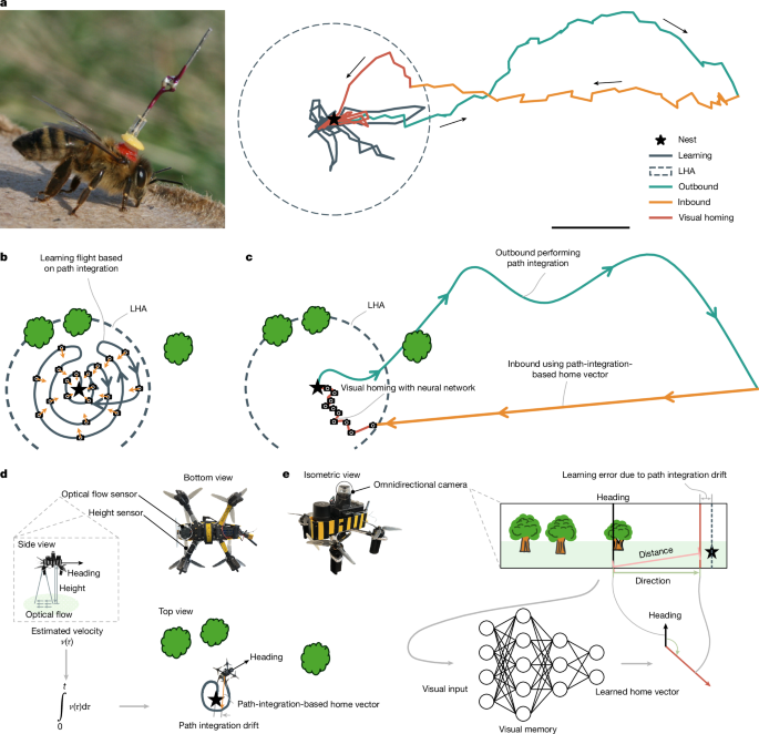
The results in Fig. 2 are based on two simulators: (1) a simplified simulator that was used to determine the ratio of the LHA versus the total navigation area; and (2) a visually realistic simulator that was used to test the visual homing with a convolutional neural network in various generated forest environments.

Simplified simulator

In this simulator, we simulate a drone flying outwards from a starting position for a given time period and then trying to return straight home. Reflecting the real experiments, we model the drone as using a noisy gyroscope measurement for updating its heading and a noisy velocity measurement for estimating its travel distance. During both the outbound and the inbound flight, the drone determines its position with the help of path integration. Owing to the noisy nature of the heading update and the velocity estimation, the path-integration-estimated position will increasingly drift from the ground-truth position. We use a Gaussian noise model for path integration drift^22,27,53. For ‘compass-less’ path integration, as performed by the real drone, the model adds noise to the heading estimate after each time step in the simulation. To this end, samples are drawn from the normal distribution \({\varepsilon }_{\psi }\sim {\mathcal{N}}(0,t{\sigma }_{\psi }^{2})\), in which t is the time in seconds. The noise is added to the actual turn rate and accumulates over time, leading to substantial heading drift: \(\hat{\psi }\leftarrow \hat{\psi }+\dot{\psi }+{\varepsilon }_{\psi }\). Furthermore, the velocity estimation noise is likewise drawn from the normal distribution \({\varepsilon }_{d}\sim {\mathcal{N}}(0,{d\sigma }_{d}^{2})\), in which d is the distance travelled in the simulation time interval. It accumulates in the position estimate of the simulated drone: \(\hat{x}\leftarrow \hat{x}+\cos (\hat{\psi })(d+{\varepsilon }_{d})\) and \(\hat{y}\leftarrow \hat{y}+\sin (\hat{\psi })(d+{\varepsilon }_{d})\). With this “path integration noise model, the simulated drone performs a 3-min outbound flight with a speed of 2 m s⁻¹. To simulate a search task, the simulated drone flies a block-like search pattern, changing direction after every 40 m. After the outbound flight, the drone attempts to fly straight home with a higher speed of 4 m s⁻¹. Every 0.5 s, the simulated drone changes its heading to point at the presumed home location. The simulation run stops when the drone estimates that it is at (0, 0). The statistics per noise setting are based on 1,000 such simulation runs. For the investigation of different noise levels, both elements of the noise model are scaled with the factors (0.1, 0.25, 0.5, 0.75, 1.0, 1.5). The sizes of the circular LHA and total flight area are then based on the 99th percentile of the distances from the home location, for both the outbound end points and the inbound end points. We also model ‘compass-based’ path integration, as performed by some robots with a magnetometer³¹ and by insects by using sky-light polarization⁴². In that case, at each time step, the simulated drone receives the actual heading perturbed by Gaussian noise: \(\hat{\psi }\leftarrow {\psi }^{\ast }+{\varepsilon }_{\psi }\). This leads to much more accurate path integration. For the simulation experiments, we selected noise settings that resulted in a similar drift to that recorded in our own experiments or in the literature (Supplementary Information Section 11). Notably, we selected σ_ψ = 0.63° and σ_d = 0.10 m to best approximate the odometry drift of our own robotic system, which gave a mean yaw drift after 100 s of 5.10° and a mean position drift after 100 m of 0.88 m.

Visually realistic simulator

The main goal of this simulator was to determine whether a convolutional neural network is able to reliably estimate home vectors from visually realistic images, using these estimates to travel to the home location within the LHA. The simulator used is NVIDIA’s Isaac Sim⁵⁴, as it allows quick acquisition of omnidirectional images. We use a photo of a meadow landscape as background image and generate a ‘forest’ by placing 40 trees from NVIDIA’s vegetation library in a 50 × 50-m area around the home location. The trees are placed uniformly into this area, while ensuring that: (1) a 5-m-radius circle around the home is free so that it is accessible; (2) trees are further away from each other than 5 m to avoid intersection; and (3) there are maximally three trees in a 10-m-radius circle around the home location to avoid too much clutter in the learning area. The experiments reported in Fig. 2 are based on ten such randomly generated forest environments.

Proposed strategy details. For the aggregate results in Fig. 2, we performed experiments in ten different environments. In each environment, we first perform a learning flight with the same learning flight pattern followed by the robot, with parameters n_loops = 6, m_points = 150 and b_spacing = 0.35 (see the ‘Learning flight’ section). As in the real robot experiments, the learning flight positions assumed by the robot are different from the actual positions owing to path integration drift. If a position risks being inside a tree, it is moved to be 0.5 m away from the landmark centre. The learning flight results in 147 images taken in a 10-m-radius area. The noisy positions and headings resulting from the path integration are used for determining the targets for the neural network learning. We train an attention network (explained later) for 150 epochs by using the Adam optimizer with a learning rate of 0.0005 and batch size of 8. We use 95% of the dataset for training and 5% for determining a validation loss. During training, rotational augmentation is used, in which each sample image and target are rotated with the same uniformly random angle from the interval [0, 2π]. After training, we simulate a homing run as follows. An omnidirectional picture is taken at the initial location. It is fed to the neural network, which determines a home vector that has both a direction and a magnitude. The vector is used in the same way as on the robot to determine a step size and direction (see the ‘Use of output’ section). When within 2 m of a tree, the desired motion vector is adapted with a basic artificial potential field method⁵⁵ to veer away from the obstacle. After executing the step, a new image is taken and the procedure is repeated. Each run ends when the simulated drone comes within 1.2 m of the home location or when it has taken 50 steps. For obtaining the aggregated results in Fig. 2, we perform homing runs at 16 locations for different distances, equally spread around a circle. If an initial position is closer to a tree than 1 m, it is moved away from the tree centre to a distance of 1 m. The initial distance is determined by the radius factor, for which 1.0 places the drone at the edge of the LHA. The investigated radius factors are (0.5, 1.0, 1.5, 2.0, 2.5).

Snapshot method. We compare the proposed strategy with a snapshot-based method³⁴. The motivation for choosing this particular snapshot method is that its performance is robust if the current view is similar enough to the snapshot. For this method, a single snapshot is taken at the home location. The simulated drone performs homing as follows: it first moves to a position to the left, right, front and back of the current position. At each displaced position, an image is taken. This image is exhaustively rotated pixel by pixel. For each rotation, the image difference D = |I_c − I_s| is determined with the home snapshot, in which I_c is the current, rotated image and I_s is the snapshot image. Per displacement, the minimal image difference min(D) is retained. Having four values for the image difference allows the simulated robot to estimate the best direction to reduce the image difference (D_x, D_y). The robot then moves 0.5 m in that direction. Although this method requires only a single snapshot at the home location, it does require many movements on the part of the robot. Moreover, exhaustive rotations are computationally expensive.

Perfect memory method. We also implemented a method that uses the same learning images as the proposed strategy but now stores them for exhaustive matching during navigation. Hence, this perfect memory method stores 147 ‘snapshots’. At each time step, the simulated robot compares the current image with all snapshot images, using the same procedure as detailed for the snapshot method—rotating the image pixel by pixel and retaining the minimal image difference (min(D)) per snapshot. After this exhaustive image matching, the k = 3 most similar snapshots are selected and the corresponding target vectors averaged to give the desired motion vector. This method is inspired by two perfect memory methods from the literature^51,52. Both of these methods are more efficient than exhaustive matching in different ways. In ref. ⁵², only four snapshots were chosen out of all snapshot images made on a grid, on the basis of an observation that more snapshots did not substantially improve homing performance. Here we included all snapshots to ensure maximal performance at the cost of more computation. In ref. ⁵¹, the navigation was purely based on left and right commands, depending on the home being visible in the left or right visual hemisphere during a real wasp’s learning flight. Here we stored real-valued target vectors, that is, with a direction and a distance, for better performance and more adequate comparison with the proposed navigation method.

Robotic platform

Robot hardware systems

The robotic platform is a custom-built quadcopter that operates autonomously, with all perception and computing handled by onboard systems without reliance on external positioning (Extended Data Fig. 1). The drone is equipped with a Raspberry Pi 4 as its primary onboard computer. A Pixhawk 6C Mini flight controller, running the PX4 autopilot firmware, manages low-level flight control. The perception system consists of several key sensors. A Raspberry Pi V2 camera fitted with a catadioptric omnidirectional lens (Kogeto Dot 360 panoramic lens) serves as the main vision sensor. For odometry, a PMW3901 optical flow sensor provides horizontal motion data, whereas a TFmini-S LiDAR rangefinder measures height for vertical positioning. These raw sensor data are combined with inertial measurement unit data by an extended Kalman filter, running on the Pixhawk, to generate the final odometry estimate (position relative to home and current heading). Furthermore, a RealSense D435i depth camera and TF-Nova range sensors are attached for some of the experiments and used only for obstacle avoidance (see the ‘Obstacle avoidance’ section). Finally, a Holybro F9P GPS module is mounted to record ‘ground-truth’ position data during outdoor experiments. Other available sensors, such as the magnetometer and barometer, are disabled for all experiments to ensure consistency.

Onboard software

The onboard software operates in a modular architecture using Docker containers. The primary vision system resides in a dedicated ‘camera container’, for which the omnidirectional camera is activated by an HTTP request. Within this container, captured images are first preprocessed using the methods detailed in the ‘Image processing’ section. Within the same container, the network then performs inference and outputs a 2D vector that represents the predicted coordinates of the home position in the current body reference frame of the drone. This vector is subsequently used to derive the desired yaw angle and distance to home, which are relayed back to the main navigation node for flight control. The ‘navigation node’ runs in a separate container using ROS2. It receives the output from the neural network as well as current state estimates (position and heading) from the PX4 autopilot⁵⁶. On the basis of this information, it sends high-level control commands back to the PX4. Sensor data are routed directly to the flight controller: optical flow data are transmitted by means of UART and distance sensor data are passed by means of I2C.

Visual homing model

Image processing

A catadioptric omnidirectional camera, which uses a convex mirror and a vertically oriented lens, captures a 360° panoramic view. As can be seen in Extended Data Fig. 3a, the raw output is an annular (ring-shaped) RGB image, in which the central and outer areas contain no useful visual information. A preprocessing pipeline is applied to each image. First, the annular region of interest is isolated using a predefined binary mask. Second, this region is unwrapped into a rectangular panorama through a linear–polar transformation, implemented with the linearPolar function from the OpenCV library. Finally, the resulting image is rotated to align with the body-frame orientation of the drone and resized to 3 × 192 × 1,800 pixels, as required by the neural network.

Data labelling

The network training uses a self-supervised learning approach in which ground-truth labels are derived directly from the onboard odometry data of the drone. As described in Extended Data Fig. 4, for each captured image, the estimated global position of the drone to home, represented by the vector \({\bf{p}}=[\begin{array}{c}{p}_{x}\\ {p}_{y}\end{array}]\), and its estimated heading (yaw), ψ_drone, are logged. The objective is to calculate a target home vector label, L, which represents the home position in the body-fixed reference frame of the drone. This vector is computed in two steps. First, the vector pointing from the current position of the drone to the home origin (0, 0) in the world frame is determined, which is simply −p. Second, this vector is transformed into the reference frame of the drone by applying a clockwise 2D rotation matrix, R(−ψ_drone), which aligns the world frame with the current heading of the drone. The final label vector L is calculated using the following operation:

The resulting components, L_x and L_y, directly represent the coordinates of the home location relative to the forward-facing perspective of the drone. This vector L serves as the ground-truth label for training the neural network.

Wind correction

Strong wind conditions (> 5 m s⁻¹ with gust >10 m s⁻¹) pose a substantial challenge during outdoor flights, forcing the drone to maintain a large tilt angle—up to 30°—to counteract the aerodynamic forces. This tilt introduces two primary issues in the captured omnidirectional images, which can provide false cues to the neural network. First, if wind conditions cause the tilt of the drone to differ from what it was during the learning phase, the learned visual cues—such as the apparent distance from landmarks to the bottom of the frame—become unreliable. This can lead to a faulty estimation of the true position of the drone, even when it is at the correct spot. Second, it causes a sinusoidal distortion of the horizon line in the unwrapped panoramic image, which in turn corrupts the perceived spatial relationships between landmarks. These problems caused by camera tilt are well known in the omnidirectional vision-based homing literature⁵⁷. To mitigate these effects, we correct the distortion by dynamically adjusting the centre point used in the linearPolar unwarping process (also see Extended Data Fig. 3d). Two methods are used to determine the necessary offset for this unwarping centre: (1) model-based correction: a linear model maps the current pitch and roll angles of the drone, obtained from the extended Kalman filter, to the required x–y offset for the unwarping centre and (2) vision-based correction: when a clear horizon is visible, it is detected in the image and used as a geometric reference to calculate the centre point that flattens the sinusoidal distortion. This vision-based method is reminiscent of the method presented in ref. ⁵⁸. Both methods have their weaknesses, so the choice between these two correction methods is made dynamically on the basis of environmental conditions. The vision-based correction is given priority in environments with a consistently visible ground horizon, as it adapts in real time to the current image and is independent of other sensor measurements that may be subject to delay. In environments in which a stable horizon is not available, the system defaults to the model-based correction, which provides sufficient reliability. Please note that, if the model-based correction relies on attitude estimates based on the inertial measurement unit, it will be susceptible to drift over time. This can deteriorate the results for long trajectories.

Neural networks

Two neural network models have been proposed for the visual homing mode: an extremely lightweight convolutional neural network (referred to as the ‘compact network’) and an only slightly larger attention-based Inception network (referred to as the ‘attention network’). The detailed architecture of these two models can be seen in Extended Data Fig. 2. The compact network is designed for high efficiency, containing four convolutional layers and a final fully connected output layer with two neurons, with a total of only 868 parameters (3.4 kB). The attention network has 10,820 parameters (42.3 kB) and is built on two custom Inception modules⁵⁹. Each module uses parallel branches with different kernel sizes, pooling and dilated convolutions to capture features at several scales. Crucially, each module also incorporates a spatial attention mechanism⁶⁰, which generates a map to reweight features and allow the network to focus on the most salient spatial regions of the image. This second, slightly deeper network is composed of the two Inception modules, two extra convolutional layers and two fully connected layers, with weights initialized using the Xavier uniform method. Both models use the tanh activation function and are designed to take panoramic colour images with a size of 3 × 192 × 1,800 pixels as input.

Use of output

The output of the network is a 2D home vector \({{\bf{h}}}_{{\rm{pred}}}=[\begin{array}{c}{h}_{x}\\ {h}_{y}\end{array}]\). which represents the predicted location of the home position in the body-fixed reference frame of the drone. This vector is directly translated into control commands, as described in Extended Data Fig. 5. The required change in heading, ∆ψ, is determined by the angle of the vector, calculated as ∆ψ = atan2(h_x, h_y), in which a positive angle corresponds to a clockwise rotation. The magnitude of the vector, d_pred = ‖h_pred‖, determines the step size (distance), s, for the next forward movement of the drone according to the linear relationship s = kd_pred + s_min, in which k is a scaling factor and s_min is the minimum distance it should take. For our experiments, we use a constant scaling factor of k = 0.13. The minimum step size, s_min, is set to 0.1 during standard tests and increased to 0.5 in windy conditions to ensure that the drone makes sufficient progress against aerodynamic forces. After rotating to the new heading, the drone moves forward a distance s. On reaching this new position, the cycle repeats with the capture of a new image. This strategy ensures larger steps when far from home and smaller, more precise steps near the target to prevent overshoot.

Experiment set-up

Environment

Experiments were conducted across a variety of indoor and outdoor environments to validate the robustness and scalability of the system (Extended Data Fig. 6). Initial algorithm validation (visual learning and homing) was performed in the 10 × 10-m CyberZoo at TU Delft, a controlled lab space with motion capture system as ground truth. Full-scale flight tests were conducted in larger, more challenging locations. To test performance in GPS-denied environments, we used two indoor hangars: the 30 × 40-m Unmanned Valley indoor facility in Valkenburg, the Netherlands (the large indoor area), which provides a large, visually structured area, and a 30 × 25-m section of the Delft Drone Initiative flight hall (the small indoor area). To test against more challenging conditions, outdoor experiments were performed in two distinct open-field environments: the outdoor test field at Unmanned Valley, a 400 × 500-m permissible flight area (the large outdoor area), characterized by natural terrain and lighting in an open field, and a 35 × 20-m tennis court in Sardinia, Italy (the small outdoor area), which provided a visually distinct, closed scene.

Learning flight

In a new environment, the drone acquires training data during a learning flight conducted in a small area around the designated home location. Because the learning flight trajectory determines the data for learning the homing vector, it has a substantial influence on the subsequent homing performance. In our experiments, we did not mimic the actual, varying honeybee learning trajectories (Supplementary Information Section 7). Given the proposed technological solution, we opted for a trajectory pattern that ensured covering a circular region around the home location. A comparison of an Archimedean spiral with a ‘wasp-like’ flight pattern^51,61 showed that the latter resulted in better homing performance, as it does not lead to the learning of spurious cues (Supplementary Information Section 6). Hence, the wasp-like pattern was used for all experiments. This pattern is generated algorithmically, starting with a classical Archimedean spiral defined in polar coordinates by the equation r = bθ, in which r is the radius, θ is the angle and the parameter b controls the distance between the arms of the spiral. The angle θ is discretized into m steps over a total of n full rotations, spanning from 0 to 2nπ. The key ‘wasp-like’ modification is a periodic mirroring of the trajectory: each time the path crosses the negative y-axis, the x-coordinates for all subsequent points are inverted. This creates a series of back-and-forth loops that expand outwards from the centre. The parameters are adjusted on the basis of the environment size; for example, for a small 10 × 10-m area, the path consists of n_loops = 4 discretized into m_points = 36 waypoints with b_spacing = 0.1, creating a learning flight with a maximum radius of approximately 2.5 m. For larger outdoor areas, the pattern is expanded to n_loops = 5 loops with m_points = 36 waypoints and b_spacing = 0.2, resulting in a learning flight with a maximum radius of approximately 6.3 m. Once learning is completed, the network is trained using one of the learning set-ups described below.

Network learning set-up

Depending on the mission constraints and resource availability (for example, time, hardware and so on), one of three distinct learning set-ups can be used: offboard, offline learning; onboard, offline learning; and onboard, online learning. Extended Data Table 1 summarizes the computational requirements and performance in one of the experiments for each set-up. Offboard, offline learning is used when a ground station with sufficient processing power (a modern CPU) and data transmission (for example, Wi-Fi, capable of transferring approximately 100 MB of data) is available. On completion of the learning flight, the raw omnidirectional images and associated labels (generated from the specific odometry data; see the ‘Data labelling’ section) are transferred to a ground station laptop. During the experiments, we used an Apple MacBook Air, with Apple M1 chip and 8 GB unified memory. The network is trained using extensive data augmentation to improve generalization, specifically by means of virtual rotation and colour augmentation (also see Extended Data Fig. 3b,c). For virtual rotation, we make use of the panoramic nature of the omnidirectional images to simulate different camera headings from a single captured frame. This is achieved by horizontally shifting the image pixels to rotate the gaze direction of the camera. For each captured image, we generate 360 new training samples by rotating the gaze in 1° increments. The corresponding label vector is recalculated for each shift to reflect the new relative heading to the home position. Subsequently, colour augmentation is applied to account for variable outdoor lighting. We duplicate each virtually rotated image and adjust its brightness by a factor sampled from U(0.9, 1.1) and its contrast by a value from U(−10, 10). For onboard, offline learning, when a ground station is unavailable or data transmission is unreliable, training is performed locally on the drone’s onboard computer (Raspberry Pi 4). To accommodate faster training with the more limited computational resources, we introduce two optimizations compared with the offboard approach. First, colour augmentation is omitted to reduce preprocessing overhead and duplication of the dataset. Second, the virtual rotation step size is increased from 1° to 5°, reducing the training dataset size by a factor of five. Despite the slower onboard processor, these optimizations ensure that the total training time remains comparable with offboard methods while maintaining successful homing performance. For missions requiring immediate execution (for example, outbound flights have to be executed less than 2 min after the learning flight), we use onboard, online learning. In this mode, training initiates in-flight immediately after the first image is captured. We use multithreaded processing on the Raspberry Pi: specific cores are dedicated to navigation and communication, whereas two cores are isolated for network training. Image capture and training happen asynchronously. Captured images are continuously appended to an image bank (stored as tensors in RAM), which serves as a replay buffer for the training thread. Given the short duration of the learning flight and the small number of images, the memory footprint is manageable, eliminating the need for a deletion policy. The training thread continuously samples batches from this buffer and applies random virtual rotation (sampled from virtual rotation step size of 1º). Training concludes exactly one minute after the learning flight ends; this interval ensures that the final learning images are sufficiently represented in the training distribution. All training configurations use the Adam optimizer with a learning rate of 9 × 10⁻⁴ and a batch size of 4. The offboard and onboard methods are trained for one epoch, whereas the online learning set-up uses a continuous rolling update strategy. All methods were validated in the CyberZoo environment, achieving a 100% success rate across all visual homing trials. Extended Data Table 1 and Fig. 3b summarize the training configuration and navigation performance for each method.

Full-flight implementation

After the learning, the forage part of the navigation strategy is implemented as a three-phase process: an outbound search, an inbound return through odometry and a final visual homing phase. During the outbound phase, the drone follows a predefined trajectory designed to cover the test area. Throughout this phase, the drone continuously updates its state estimate (position and heading) relative to its starting point using onboard odometry. Although simple paths are used for most experiments, more complex patterns, such as a grid search, are also used in some indoor environments to simulate real-world applications such as search and rescue. Once the outbound trajectory is complete, the drone switches to the inbound phase. The flight controller is commanded to return to the home coordinates (0, 0) based on the current odometry estimate. The drone executes a direct, high-speed flight towards this estimated home position. On reaching the odometry-based goal, the final visual homing phase is initiated. Owing to the expected accumulation of odometry drift, the estimated position of the drone does not perfectly align with its true starting location. Therefore, the system switches to the neural-network-based visual control strategy, described previously in the ‘Use of output’ section, to perform the final, precise approach to the home location. In all of our experiments, the home location is not visible by itself, so we stop the experiments when the drone arrives close enough to the home location. A success is hereby defined as the drone ending up within 0.5 m of the home location. Some example trajectories of these full flights can be seen in Extended Data Figs. 7 and 8.

Obstacle avoidance

Inspired by Wedgebug⁶², we implemented a reactive detect-and-avoid system based on a finite-state machine, in which the sensing hardware evolved to match the computational constraints of the onboard Raspberry Pi. Initial experiments used an Intel RealSense D435i depth camera with the depth map segmented into left, centre and right average-depth bins, whereas the later experiments used three TF-Nova LiDAR sensors monitoring a 1° × 14° field of view for each sector. The avoidance logic interrupts the primary navigation loop whenever the front distance d_front drops below a predefined stopping threshold d_stop, at which point the evasion trajectory is calculated on the basis of the specific flight phase.

For the learning, outbound and inbound phases, the core avoidance logic is identical. The system monitors the left, centre and right sectors. If the centre is blocked, the drone determines which side (left or right) is clear, rotates in that direction and executes a forward movement of d_evade. Immediately after this evasion, it realigns its yaw to face the original target waypoint. If all three sectors (left, centre and right) are blocked, the system triggers a panic mode: the drone rotates by a larger angle ψ_drone, travels a distance of d_panic and attempts to resume navigation by realigning to the target waypoint again in this new position. However, if after n_attempts the same target waypoint is still not reached, the next movement differs by phase:

• Learning phase: if the point remains unreachable after n tries, the system skips it, takes an image and records the label at the current position and heading and proceeds to the next learning waypoint.

• Outbound phase: if blocked, the system skips to the next outbound waypoint. If the outbound path is completed, it automatically switches to the inbound phase.

• Inbound phase: the system persists in trying to reach the odometry coordinates (0, 0). However, if the drone is stuck but within 2 m of the odometry coordinates (0, 0), it aborts the inbound flight and immediately switches to visual homing.

During the homing phase, the detection logic (checking left/centre/right) and the evasion movement d_evade remain the same. However, the post-evasion behaviour is different: the drone does not realign to the previous target. Instead, it simply captures a new image at its current position, queries the network for a new prediction, rotates to this new predicted heading and restarts the obstacle detection and evasion loop again.