Long-term editing of brain circuits using an engineered electrical synapse

Design of the Cx34.7 and Cx35 mutant library

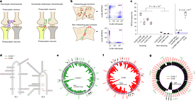
A semi-rational design approach was used to design the mutant library. Sequence alignments between the M. americana connexins and the connexins for which the most structure–function data existed (Cx26, Cx32, Cx36, Cx40 and Cx43) were performed in ClustalW. Sites identified by previous studies as conferring specificity for docking were used, as well as those identified by homology modelling from the structures of Cx26 (ref. ⁵⁶). Specifically, we primarily focused on residues in the extracellular loops: four residues at the interface in EL2, KEVE/KDVE (M. americana Cx34.7 and Cx35), and one residue in EL1. The homologous residues in other connexins had been demonstrated to be highly tolerant to mutations and critical for docking specificity⁵⁷. Mutations were modelled in Swiss PDB Viewer using homology models of Cx34.7 and Cx35 from a Cx26 and Cx32 interface structure so as not to create mutations with obvious steric hindrance. A wide range of substitutions were made for these five residues of interest, including those intended to introduce compatible electrostatic interactions, as well as less likely candidates. Mutations were also created that targeted other residues nearby and/or adjacent to these five for which there was some published evidence that they contributed to docking specificity. However, our semi-rational approach was such that not as many variants were evaluated for these more distal site mutations; mutations made in those sites were more conservative with regards to the steric and electrostatic properties of the change.

Construct cloning and preparation

The initially acquired M. americana Cx34.7 and Cx35 cDNA constructs did not express efficiently in HEK293FT cells. Thus, connexin gene information was procured from the National Center for Biotechnology Information (NCBI) and the Ensembl genome browser. The human codon-optimized genes were ordered from Integrated DNA Technology (IDT) as gBlocks Gene Fragments. To generate constructs for transient transfection of HEK293FT cells, genes were subcloned into BamHI-digested and SacI-digested mEmerald-N1 (Addgene, 53976) and piRFP670-N1 (Addgene, 45457) vectors using In-Fusion cloning (Takara Bio), which resulted in connexin fluorescent fusion proteins, specifically with the fluorescent proteins adjoined to the connexin carboxy terminus. Mutant constructs were generated by using overlapping primers in standard Phusion polymerase PCR reactions to facilitate site-directed mutagenesis.

The Gateway recombination (Invitrogen) system was used to generate all Cx36, Cx34.7, Cx35, WT and mutant protein C. elegans expression plasmids. For PCR-based cloning and subcloning of components into the Gateway system, either Phusion or Q5 High-Fidelity DNA polymerase (NEB) was used for amplification. All components were sequenced in the respective Gateway entry vector before combining components into expression plasmids via a four-component Gateway system⁵⁸. The different connexin versions were introduced into pDONR221a using a similar PCR-based strategy from plasmid sources^8,59,60. Cell-specific promoters were introduced using the pENTR 50-TOPO vector (Invitrogen) after amplification from genomic DNA or precursor plasmids. Transgenic lines were created by microinjection into the distal gonad syncytium⁶¹ and selected on the basis of expression of one or more co-injection markers: Punc-122::GFP or Pelt-7::mCherry::NLS.

Cell culture

HEK293FT cells were purchased from Thermo Fisher Scientific (R70007) and were maintained according to the manufacturer’s instructions. In brief, cultures were grown in 10-cm tissue culture-treated dishes in high-glucose DMEM (Sigma Aldrich, D5796) supplemented with 6 mM l-glutamine, 0.1 mM MEM non-essential amino acids and 1 mM MEM sodium pyruvate in a 5% CO₂, 37 °C incubator. Cells were passaged by trypsinization every 2–3 days or until 60–80% confluency was reached. The cell line identity was not validated beyond the manufacturer’s certification of authenticity, and it was not tested for mycoplasma contamination. HEK293FT cells are not included in the list of commonly misidentified cell lines published by the International Cell Line Authentication Committee.

Transient transfection

HEK293FT cells were plated in 10 μg ml^–1 fibronectin-coated multiwell dishes to achieve about 75% confluency after overnight incubation. For transfection, 250 ng DNA was combined with polyethylenimine (PEI) diluted in Opti-MEM in a 1:3 ratio (DNA (µg) to PEI (µl)) and incubated at room temperature for 10 min. Following incubation, PEI–DNA complexes were added dropwise to wells of the plated cells. Treated cells were then incubated at 37 °C for 16–18 h, followed by a change in the medium. Expression of the connexin–fluorescent protein constructs were evaluated at 24 and 48 h after transfection by widefield or confocal microscopy and western blotting.

FETCH

FETCH analysis is fundamentally a two-component system (Extended Data Fig. 1). To complete FETCH analysis, replica multiwell plates with HEK293FT cells were transfected with either of the two components being evaluated. The media of transfected wells were changed 16–18 h after transfection and cells were trypsinized. Next, HEK293FT cells expressing experimental connexin counterparts were combined. The entirety of combined samples was then plated onto new, 10 μg ml^–1 fibronectin-coated wells of the same size, which resulted in hyperdensity and overconfluency. Following co-plating, samples were incubated for around 20–24 h, which allowed cells to make contacts and to potentially generate and internalize dually labelled gap junctions. Samples were then trypsinized, resuspended in PBS with 10 U ml^–1 DNAse and fixed with paraformaldehyde (PFA; final concentration of 1.5%). Co-plated samples in 96-well plates were resuspended to a final volume of around 150 µl, whereas samples from 24-well plates were resuspended to a final volume of about 600 µl.

Flow cytometry data were collected on a BD FACSCanto II (2-colour experiments and high-throughput 96-well plates; 488 nm and 633 nm lasers), which uses BD FACSDiVa software. Samples were analysed in two selection gates before evaluation of fluorescence. First, presumable HEK293FT cells were identified by evaluating sample forward versus side scatter area. Next, single cells were selected by evaluating cells that maintained a linear correlation of forward scatter height to forward scatter area. Finally, the fluorescence profiles of each sample were generated.

Automated FETCH output processing pipeline

Each FETCH experiment produces *.fcs files that contain all the channel data for fluorescence in the sample. Our automated pipeline loads these files and extracts forward scatter-area (FSC-A), side scatter-area (SSC-A) and forward scatter-height (FSC-H). Depending on the machine used, we either loaded the green channel as 1-A or as FITC-A. For the red channel, we had two options (APC-A (iRFP670) and PE-A (mApple)) or just one (5-A(iRFP670)). Next, our code produces two matrices containing SSC-A with FSC-A, and FSC-A with FSC-H, respectively.

Our first gate was drawn on the FSC-A versus SSC-A axes to exclude cellular debris that clustered in the lower left corner and the cells that saturated the laser (at the maximum of both axes). On a FSC-A versus SSC-A plot, the cellular debris usually is smoothly transitioning into the population of intact cells; therefore, we used a Gaussian kernel density estimator with the estimator bandwidth selection defined by the Scott’s rule to draw contours around the data in the SSC-A versus FSC-A matrix. We next used a set of heuristics to determine which of the contour lines should be used to define the first gate. Specifically, cellular debris usually clusters below 25,000 on both axes; therefore, any contour that included values at or below this value was excluded. Similarly, any contour within 1,000 of the maximum value of each axis was also excluded. Of the remaining contours, the largest one was selected and an oval equation was fitted to the points defining that contour to attenuate occasional protrusions that tap into the cellular debris population in rare cases. The fitted oval became the first gate.

For all the elements inside the first gate, a second gate was drawn in the axis of FSC-A and FSC-H to exclude non-single cells. For the second gate, first we fit a line to all the points. Next, for each point we identified a norm to the fit line and a standard deviation of all such norms. Using this standard deviation, we defined a second gate that was four standard deviations away from the fitted line on both sides and excluded all the points outside this gate (Extended Data Fig. 1c).

After applying the first two gates, we plotted the data with the red fluorophore on the y axis and the green fluorophore on the x axis. If a sample contained more than two fluorescent signals, the last gate was drawn for each possible combination. As some readings were below zero owing to fluorescence compensation, we shifted all the data points by the smallest value along both axes and then took a natural log of fluorescence levels. To achieve the optimal bandwidth for the kernel density estimation, we ran a cross-validation grid search algorithm on the points in the log space. Then we fit a Gaussian kernel density with the bandwidth estimated to obtain density contours. For properly expressing samples, we expected a large population of non-transfected cells in the bottom left quadrant of the plot, a population of cells strongly expressing the red fluorophore along the y axis and a population of cells strongly expressing the green fluorophore along the x axis (Extended Data Fig. 1d). We anticipated that the autofluorescence does not exceed 500 on either axis; therefore, the non-transfected population was defined to be below this value along both axes. To draw a tighter bound on the non-transfected population, we chose the first contour for which the mean kernel density estimate (k.d.e.) value was at or above the 60th quantile (identified as a generalizable heuristic value) of the distribution of k.d.e. values in the largest contour (at or below the autofluorescence cutoff). The top-most point of the tight contour defined the horizontal gate and the right-most point as the vertical gate, thereby separating the plot into four quadrants.

The upper-left quadrant Q1 corresponded to the cells expressing just the red fluorophore, the upper-right quadrant Q2 represented dual-coloured cells, the lower-right quadrant Q3 the cells expressing just the green fluorophore and the lower-left quadrant Q4 represented non-transfected population. The FETCH score is defined as the proportion of transfected cells that were dual-coloured: 100 × (Q2/(Q1 + Q2 + Q3)).

As we were expecting approximately equal expression levels of each fluorophore, if the number of cells in Q1 was two or more times larger or smaller than the number of cells in Q3, the FETCH score was classified as ‘dubious’ and marked accordingly in the output table. The ‘dubious’ label was also given to samples that had fewer than 500 cells total after the application of the second gate and to the samples that failed at any of the steps in the pipeline (usually due to poor expression or the absence of cells in the sample). The code for this pipeline is available from GitHub (https://github.com/carlson-lab/FETCH).

In vitro screening of Cx34.7 and Cx35 mutants for docking selectivity

For homotypic docking screening analysis, five FETCH replicates were obtained for each mutant. These scores were benchmarked against scores for Cx36 with Cx45 (FETCH = 1.2 ± 0.1%, n = 54 replicates). For our heterotypic docking screening analysis, five replicates were obtained for each mutant pair. These scores were then benchmarked against scores for WT Cx34.7 with Cx35 (FETCH = 14.7 ± 0.4%, n = 49 replicates).

To quantitatively determine whether a connexin pair docked, we determined FETCH scores for the dual fluorescence of cells under conditions in which docking was not anticipated. These conditions included pairs of connexins previously established to not show docking (Cx36 and Cx45 (FETCH = 0.7 ± 0.0%, n = 59 replicates), homotypic Cx23 (FETCH = 0.9 ± 0.4%, n = 6), Cx36 and Cx43 (FETCH = 1.2 ± 0.2%, n = 10)) and under conditions for which cells were transfected with cytoplasmic fluorophores rather than tagged connexins (FETCH = 4.4 ± 0.6%, n = 17). These 92 FETCH scores were used as the known-negative distribution. FETCH scores from each experimental condition were then compared against the known-negative distribution using a one-tailed t-test, with an α threshold that was Bonferroni-corrected for the total number of experimental conditions tested (n = 21, producing an α = 0.05/21). These FETCH replicates were independent of the replicates used for our screening analysis. Statistics are reported as mean ± s.e.m. values, and only uncorrected P values are reported throughout.

Confocal imaging analysis of gap junction partners

For imaging of putative gap junction partners, different populations of HEK293FT cells were transfected with counterpart connexin proteins, incubated and combined as described for FETCH analysis. Combined samples of HEK293FT cells were plated onto 10 μg ml^–1 fibronectin-coated 35-mm, glass-bottom Mattek dishes (P35GC-1.5-14-C). Cells were imaged at about 20 h after plating. Images were acquired on a Leica SP5 laser point-scanning inverted confocal microscope using Argon/2, HeNe 594 nm and HeNe633nm lasers, conventional fluorescence filters and a ×63, HCX PL APO W Corr CS, NA: 1.2, water, DIC, WD: 0.22 mm, objective. Images were taken with 1,024 × 1,024-pixel resolution at a 200 Hz frame rate.

For assessing Cx34.7(M1)–Cx35(M1) expression in vivo in C. elegans, we imaged strain DCR8669 olaEx5214 (Pgcy-8::Cx34.7(E214K,E223K)::GFP;Pttx-3::Cx35(K221E)::mCherry;Punc-122::GFP). Animals at the L4 stage were mounted in 2% agarose in M9 buffer pads and anaesthetized with 10 mM levamisol (Sigma). Confocal images were acquired using dual Hamamatsu ORCA-FUSIONBT SCMOS cameras on a Nikon Ti2-E inverted microscope using a confocal spinning disk CSU-W1 system, 488 nm and 561 nm laser lines and a CFI SR HP PLAN APO LAMBDA S ×100 C SIL objective. Images were captured using NIS-ELEMENTS software, with 2,048 × 2,048-pixel resolution, 16-bit depth, 300 nm step size, 200 ms of exposure time and enough sections to cover the entire depth of the worm.

Protein modelling pipeline

Our protein modelling pipeline is based on a previously published methodology³⁴ and integrates five components: (1) homology model generation; (2) embedding of proteins in a lipid bilayer and aqueous solution; (3) protein mutagenesis; (4) short-timescale energy minimization protocol incorporating explicit solvent and bilayer effects; and (5) residue-wise energy calculation. The code for our model is available from GitHub (https://github.com/carlson-lab/VMD-and-NAMD-Connexin-Protein-Simulation-Protocol).

Homology modelling

We initially tested five homology modelling software suites: Robetta, SwissModel, Molecular Operating Environment (MOE; Chemical Computing Group, H3A 2R7, 2021), I-Tasser and Phyre2 (refs. ^{62,63,64,65,66,67,68,69,70}). A quality assessment suite, MolProbity^71,72,73, revealed that Robetta models outperformed the rest, on the basis of a set of standard metrics (Ramachandran plot outliers, clashscore, poor rotamers, bad bonds or angles, among others). As our aim was to model the extracellular loops responsible for connexin hemichannel docking, we picked all the resolved connexin structures that possessed a high degree of extracellular loop homology to our connexin of interest as the inputs for Robetta. The top homologue hits were generally the same for the three connexins of interest: Cx26 bound to calcium (Protein Data Bank (PDB) ID: 5ER7.1)⁷⁴; human Cx26 (calcium-free) (PDB ID: 5ERA)⁷⁴; structure of Cx46 intercellular gap junction channel at 3.4 Å resolution by cryogenic electron microscopy (PDB ID: 6MHQ)³³; structure of Cx50 intercellular gap junction channel at 3.4 Å resolution by cryogenic electron microscopy (PDB ID: 6MHY)³³; and structure of the Cx26 gap junction channel at 3.5 Å resolution (PDB ID: 2ZW3)⁵⁶. The Cx34.7 and Cx35 WT sequences had the greatest homology degree with the 6MHQ structure, whereas Cx36 was most homologous to 5ER7.1. We generated three WT hemichannels for Cx34.7, Cx35 and Cx36.

System assembly

Next, we assembled hemichannels into homotypic and heterotypic gap junctions, embedded them in two palmitoyl-oleoyl-phosphatidylcholine membrane double bilayers, solvated them in water and added appropriate ion concentrations for the extracellular and two intracellular compartments. The primary software suite used for this modelling step was VMD^75,76. We also used CHARMM GUI to generate the naturalistic model of a region of a double bilayer^{77,78,79,80,81}. Membrane components were then selected in appropriate proportions to resemble experimentally derived data from a neuronal axonal membrane.

Specifically, as Robetta was unable to model the full gap junction, we merged hemichannels into full homotypic or heterotypic gap junctions in a semi-automated way. First, to make homotypic gap junctions, we loaded the two homology models for a hemichannel. We then aligned them using the centre of mass of the extracellular loops. To make heterotypic gap junctions, we created a homotypic gap junction for each hemichannel, aligned the extracellular loops for the two homotypic gap junctions, then removed an opposing hemichannel from each homotypic gap junction (leaving the two different hemichannels aligned). Next, using the constructed gap junction, we aligned two pre-made membrane bilayers with the centre of mass assigned as each embedded hemichannel. We then removed membrane molecules that overlapped the hemichannel or the hemichannel pore. Next, we solvated the system in water and removed water that overlapped the lipid bilayer. Extracellular water was then separated to a new file, where Na⁺ ions [130 mM], K⁺ ions [5 mM], Cl^– ions [150 mM] and Ca²⁺ ions [2 mM] were added to produce concentrations mirroring the extracellular environment of mammalian neurons⁸². Finally, Na⁺ ions [12 mM], K⁺ ions [125 mM], Cl^– ions [10 mM] and Ca²⁺ ions [0.0001 mM] were added to the intracellular space to mirror the intracellular environment of mammalian neurons, and the files containing the embedded connexin hemichannels and extracellular water were merged, which generated solvated hemichannels at a pH of 7.2–7.4. Notably, these stages were automated to produce a streamlined progression from a protein-only hemichannel model to a fully embedded gap junction model ready for subsequent simulation and/or mutagenesis.

Mutagenesis

We developed a Python command-line tool that uses VMD to generate mutation configuration files for subsequent molecular dynamics simulation. Here we simply specified the connexin hemichannels of interest and the position at which a specific mutation should be introduced.

Short-timescale energy minimization protocol incorporating explicit solvent and bilayer effects

Next, we minimized atomic energies, equilibrated the system and ran the stable system in a production simulation run. Specifically, molecular dynamics simulation was performed using NAMD⁸³ and a CHARMM36 force field. Our approach was divided into four steps:

1. 1)

   Melt lipid tails while keeping remaining atoms fixed (simulate for 0.5 ns, NPT, 300 K).

2. 2)

   Minimize the system (NVT, 300 K), then allow the bilayers and solutions to take a natural conformation while keeping the gap junction fixed (split in two stages to accommodate the reduction in volume of the relaxing system; simulate for 0.5 ns in total, NVT, 300 K, with harmonic positional restraints on the protein).

3. 3)

   Release the gap junction and equilibrate the whole system (simulate for 0.6 ns, NVT, 310 K, 1 atm, using Langevin dynamics).

4. 4)

   Run the minimized and equilibrated system in a production run (simulate for 0.5 ns, 1-fs step, NPT, 310 K).

Although molecular dynamics simulation (step 4) is highly reliant on the input file provided by the System Assembly process, these steps render the simulation more robust to modelling imperfections. For example, the membrane model developed though System Assembly is rigid and has the potential to behave like a solid rather than like a liquid. Thus, melting the lipid tails encourages the model to embody a liquid. Similarly, many atoms in the input file may have unnatural initial energies, such that if they are all released at once, they would start moving at high velocities and the simulation would fail. Therefore, bringing the system to a local energy minimum increases stability. Removing constraints on the water and lipids enables them to surround the gap junction in a naturalistic form. Finally, releasing the constraints on the gap junction enables it to take the most energetically stable conformation given the environment.

Energy calculation

To predict the residues that play a prominent part in docking, we quantified all non-bonding interactions between the two connexin hemichannels at key residues on the extracellular loops. Output from the molecular dynamic simulation was loaded into the VMD NAMD Energy plugin. We then calculated non-bonding energies for all residues on each hemichannel that were within 12 Å from at least one residue on the other hemichannel. For each residue pair, we then averaged energies across the 250 simulation frames.

Characterizing gap junction biophysical properties using Xenopus oocytes

DNA sequences encoding Cx34.7(WT)-mEmerald, Cx34.7(M1)-mEmerald, Cx35(WT)-mApple and Cx35(M1)-mApple were cut out from the plasmids used for our mouse studies (see below) using BamH1 and ECoR1 and then cloned into the pXMX_T3(+) Xenopus oocyte expression vector at identical restriction sites. The newly generated plasmids were linearized by cutting with NgoMIV to serve as templates for in vitro synthesis of complementary RNAs (cRNAs). Capped cRNAs were synthesized using a mMessage mMachine T3 Transcription kit (AM1348, ThermoFisher Scientific). Each cRNA injection solution was a mixture of a specific cRNA and a Cx38 antisense oligonucleotide (5′-GCTTTAGTAATTCCCATCCTGCCATGTTTC-3′, 100 ng µl^–1).

In preliminary experiments with Cx34.7^WT and Cx35^WT cRNAs injected at an identical concentration (900 ng µl^–1), we observed much larger I_j values in a homotypic gap junction of Cx35(WT) than one of Cx34.7(WT) under identical experimental conditions. Moreover, there was a larger cytotoxic effect (oocytes dying) with Cx35(WT) but not Cx34.7(WT). Therefore, in the final injection solutions used for the main experiments presented in this study, the concentrations of Cx34.7^WT-mEmerald and Cx34.7^M1–mEmerald cRNAs were 900 ng µl^–1, whereas those of Cx35^WT-mApple and Cx35^M1-mApple cRNAs were 90 ng µl^–1. Approximately 50.6 nl of the mixture was injected per oocyte using a Drummond Nanoject II injector (Drummond Scientific). Injected oocytes were incubated in ND96 solution (96 mM NaCl, 2 mM KCl, 1.8 mM CaCl₂, 1 mM MgCl₂ and 5 mM HEPES (pH 7.5)) inside an environmental chamber (15 °C) before being paired. Oocytes were paired 20–24 h after Cx35^WT and Cx35^M1 cRNA injections, but 68–72 h after Cx34.7^WT and Cx34.7^M1 cRNA injections. To closely match experimental conditions between related groups, oocytes from one frog were used to analyse homotypic gap junctions of Cx34.7(WT) and Cx34.7(M1), whereas oocytes from another frog were used to examine homotypic gap junctions of Cx35(WT) and Cx35(M1). Furthermore, an identical batch of oocytes from a third frog was used to investigate heterotypic gap junctions of both Cx34.7(WT)–Cx35(WT) and Cx34.7(M1)–Cx35(M1). The vitelline membrane of the oocyte was removed using a pair of no. 5 Dumont tweezers (500342, Word Precision Instruments) during the pairing process. Paired oocytes were incubated in ND96 solution for 12–24 h at room temperature (20–22 °C) before electrophysiological recordings. Voltage–clamp recordings were performed using two Oocyte Clamp amplifiers (OC-725C, Warner Instruments) in the high-side current measuring mode. In the electrophysiological experiments, we applied a series of membrane voltage steps (–150 mV to +90 mV at 10-mV intervals, 7 s in duration) to one oocyte from a holding voltage of −30 mV while holding the other oocyte constant at −30 mV to record transjunctional currents (I_j). A pre-pulse (–30 mV) was applied from the holding voltage before each voltage step so that the stability of the recordings could be monitored by the induced I_j. Instantaneous current (I_inst) and steady-state current (I_ss) were defined as the peak I_j at the beginning of each V_j step and as the averaged I_j during the last 2 s of the V_j step, respectively. Details of the experimental and data analysis procedures can be found in our previous publications^35,36.

Generation and validation of Cx43 and Cx45 double-knockout HEK293FT cells

Connexin double-knockout HEK293FT cells were produced by the Duke Functional Genomics Core Facility using CRISPR–Cas9 technology. Specifically, insertion and/or deletion mutations were introduced via CRISPR–Cas9 in the Cx43 and Cx45 sequences to induce frameshifts in the Cx43 (GJA1) and Cx45 (GJC1) DNA sequence, which results in premature translation termination (Extended Data Fig. 5a–c). Specific mutations were identified through DNA sequencing and evaluation of sequence chromatograms (exported as encapsulated postscript (.eps) files) in ApE Plasmid editor⁸⁴. To confirm Cx43 and Cx45 knockout, three double-knockout HEK293FT monoclonal cell lines were isolated and expanded for evaluation by western blotting. Cells were collected in ice-cold PBS (Gibco, 10010031) enriched with protease and phosphatase inhibitors 1:100 (Sigma-Aldrich, P8340 and P5726). Cells were then centrifugated at 1,000g for 5 min at 4 °C to remove PBS, and the pellet was sonicated twice for 30 s (20% output power) in ice-cold lysis buffer (Phosphosolutions, NC1671658) enriched with protease and phosphatase inhibitors 1:100 (Sigma-Aldrich, P8340 and P5726). Cell lysates were kept on ice for 30 min and then centrifugated at 14,000g for 30 min at 4 °C. Lysate supernatants were collected, and total protein concentrations were measured using a bicinchoninic acid assay (Thermo Fisher Scientific, 23228 and 1859078). Next, 40 μg of total protein was denatured at 95 °C for 5 min in LDS sample buffer (7 µl per sample) (Thermo Fisher Scientific, NP0007) and sample reducing agent (3 µl per sample) (Thermo Fisher Scientific, NP0009). The denatured samples were then separated using Novex Tris-Glycine gels 4–20% (Thermo Fisher Scientific, XP04200BOX) and electrophoresis at 125 V for 10 min and 150 V for around 1 h, then transferred to polyvinylidene fluoride membranes (Thermo Fisher Scientific, 88520) overnight at 0.04 A. Membranes were blocked with 5% dry non-fat milk (Blotting-Grade Blocker, Bio-Rad, 1706404) in PBST (0.1% Tween-20) for at least 2 h at room temperature and next incubated overnight at 4 °C with the following antibodies in blocking solution: anti-Cx43 (Cell Signaling Technologies, 3512, 1:1,000) and anti-Cx45 (Abcam, ab316742, 1:1,000). GAPDH was measured after the protein of interest (Cx43 or Cx45) as control (anti-GAPDH, Abcam, ab181602, 1:5,000). After incubation with the primary antibody, this was removed and blots were washed in PBST 0.1% (3 washes, 15 min each) at room temperature, following incubation with horseradish-peroxidase-labelled secondary anti-rabbit IgG antibody (Cell Signaling Technologies, 7074) for 1 h at room temperature. Membranes were washed in PBST 0.1% to remove the secondary antibody (3 washes, 15 min each). Immunoreactive bands were visualized with SuperSignal West Pico PLUS Chemiluminescent substrate (Thermo Fisher Scientific, 34578) and detected using a ChemiDoc Imaging system (Bio-Rad, 12003153). Bands were analysed with ImageJ. For each protein studied, the ratio was calculated by dividing the densitometric value of the protein of interest by the correspondent GAPDH value × 100 (Extended Data Fig. 5).

PCR confirmation of Cx43 and Cx45 knockouts

Genomic DNA from HEK293FT double-knockout cell line clones of 405, 412 and 422 was extracted using a KAPA NGS DNA extraction kit (Roche, 09189823001), and PCR was performed using Invitrogen Platinum super Fi PCR master mix (12358010) following the manufacturer’s instructions. PCR products were prepared by adding a DNA stain (APEBIO, ab743) and then separated in 1% agarose gel (Bio-Rad, 1613102) in TAE buffer (Bio-Rad, 1610743) at 100 V for about 30 min. DNA fragments were detected using a ChemiDoc Imaging system (Bio-Rad, 12003153).

WT and connexin double-knockout HEK293FT cultures for patching experiments

WT HEK293FT cells were purchased from Thermo Fisher Scientific (R70007). Connexin double-knockout HEK293FT cells were generated as described above. Cells were maintained according to the manufacturer’s instructions as noted above.

Glass coverslip preparation

In brief, 12-mm German glass coverslips (NeuVitro, GG-12-15-fibronectin) were first pretreated with acetone for 20 min with shaking. Next, they were washed 3 times for 10 min in 70% ethanol with shaking and stored in 70% ethanol before use. Once needed, each coverslip was washed 6 times with cell-culture-grade deionized water to remove any ethanol remnants. For the patching experiments, coverslips were then coated using 1:100 fibronectin (Sigma-Aldrich, F1141-2MG) (stock at 1 mg ml^–1) in poly-d-lysine (Gibco, A38904-01) (stock at 0.1 mg ml^–1 in PBS) for 1 h at room temperature. After coating, the solution was aspirated and the coverslips were left to dry in a cell culture hood, uncovered, for 1–2 h.

Sample preparation for paired cell recordings

For the recording experiments using non-transfected cells, HEK293FT or connexin double-knockout HEK293FT cells were grown in 10 cm tissue-culture-treated dishes and seeded onto the coverslips, at the same density conditions used for all patching experiments (35,000 cells per well in total), the day before the recording. To evaluate connexin proteins, connexin double-knockout HEK293FT cells were seeded with no antibiotic cell culture medium, and the next day they were transfected using Lipofectamine 2000 transfection reagent (Thermo Fisher, 11668027) at a Lipofectamine 2000 to DNA ratio of 2.5–1.9:1. (0.8–1 μg cDNA to 1.9–2 µl Lipofectamine). Opti-MEM (Gibco, 31985070) medium was used following the Lipofectamine 2000 protocol. Medium was changed after 4 h to remove the transfection reagent. For each patching condition, 4 or 20 h after transfection, cells were detached, counted and re-seeded in equal amounts of cells from each fluorescent condition (35,000 cells per well in total) onto a precoated glass coverslip in a 24-well plate (see the section above for coverslip preparation). The cells were left to form gap junctions overnight and recordings were conducted the following day. These patching experiments were performed using the construct cloning and preparation procedures described above, with minor changes. In brief, for the Cx34.7(M1)–Cx35(M1) and Cx36–Cx36 patching conditions tested, cells expressed either mEmerald or mCherry. For 2 out of the 23 connexin double-knockout HEK293FT negative control experiments, we used cell pairs in which one cell expressed mEmerald and the other expressed mCherry. Finally, we used only one fluorescent tag for the Cx34.7(M1)–Cx34.7(M1) or Cx35(M1)–Cx35(M1) experiments (mEmerald and mCherry respectively).

Paired HEK293FT cell recordings

Glass coverslips with adhered WT or connexin double-knockout HEK293FT cells were placed into a recording chamber on an upright fluorescent microscope (Scientifica). The chamber was filled with extracellular solution (ECS) at room temperature (21–24 °C). The ECS contained the following factors (in mM): 5.4 KCl, 1 CaCl₂, 140 NaCl, 5 HEPES, 1.8 MgCl₂ and 5 glucose; pH was adjusted to 7.4 with NaOH, with an osmolarity of 310–320 mOsm. Patch pipettes were pulled using a micropipette puller (Sutter Instruments P1000) and filled with intracellular solution containing the following factors (in mM): 135 CsCl, 0.5 CaCl₂, 2 MgCl₂, 5.5 EGTA, 5 HEPES, 3 MgATP, 2 Na₂ATP; pH was adjusted to 7.2 with CsOH, with an osmolarity of 290 mOsm. The patch pipette resistance was in the range of 2–4 MΩ. Isolated cell pairs were selected for dual whole-cell voltage clamp experiments.

To study transjunctional currents between cell pairs, the following protocol was applied in voltage clamp. A series of square voltage pulses (stepped up from −160 mV to +70 mV in 10-mV increments) was alternated between the two cells. While the first cell received the pulses, the second cell was held at −45 mV to measure the transjunctional current. This procedure was repeated for both cells.

Analysis of transjunctional current

All current traces were filtered using Clampfit 11.4 (Molecular Devices). The baseline current was measured 500 ms before the voltage pulse. The current for each 200 ms voltage step was then determined as the difference between the current recorded during the last 50 ms of each step and this baseline current. The relationship between this current and transjunctional voltage was determined for each cell using Pearson correlation analysis, and the values were averaged across cells in a cell pair (Extended Data Fig. 6). The current at the +70 mV step was extracted for each cell and averaged across the pair to determine the maximum transjunctional current used for analysis.

To test Cx36, we plated cells expressing red or green fluorescent proteins. Because Cx36 shows homotypic docking, we patched fluorescent cell pairs irrespective of their colour. To test Cx34.7(M1)–Cx35(M1), we selected and patched pairs for which one of the cells was clearly labelled by green fluorescent protein and the other cell was labelled by red fluorescent protein. We also selected and patched pairs for which both cells were labelled by both fluorophores. Visual inspection at multiple views enabled us to separate out these experimental pairs on the basis of high confidence that one of the cells in a pair was not labelled by both green and red fluorescence (Extended Data Fig. 6). To test Cx34.7(M1) or Cx35(M1), we patched cell pairs expressing a single fluorophore.

Statistical analysis of HEK293FT whole-cell recording data

We compared untransfected WT HEK293FT cell pairs to connexin double-knockout HEK293FT cell pairs. Next, the maximum transjunctional voltage recorded from connexin double-knockout HEK293FT cell pairs transfected with connexins was compared with that from a connexin double-knockout HEK293FT cell pair control group using a one-tailed Wilcoxon rank-sum test, followed by a FDR correction. We chose one-tailed testing here because we were specifically evaluating whether the expression of our mutant proteins increased current above the baseline current observed in the connexin double-knockout HEK293FT cell pairs. Notably, in contrast to the published methodology using HEK293 cells³⁷, knocking down Cx43 and Cx45 did not completely abolish electrical coupling between HEK293FT cells. Indeed, in our preliminary experiments, we observed electrical coupling in 1 out of 10 connexin double-knockout HEK293FT cell pairs (as indicated by a transjunctional voltage × current relationship > R² = 0.75, Pearson correlation). In our main experiments, we observed coupling in 6 out of 34 of our negative control pairs (5 out of 23 connexin double-knockout HEK293FT cell pairs and 1 out of 11 of the pairs that expressed Cx34.7(M1)–Cx35(M1) but did not exhibit dual fluorescence in both cells; Extended Data Fig. 6b). In our post hoc testing, we observed a significantly higher proportion of coupled cells in our two positive control groups (7 out of 10 Cx36–Cx36 cell pairs, χ² = 10.2 and P = 0.001 compared with the pooled negative controls, chi-squared test; 7 out of 10 Cx34.7(M1)–Cx35(M1) that exhibited dual fluorescence in both cells, χ² = 10.2 and P = 0.001). These findings increased our confidence that this mammalian cell system could be used to test Cx34.7(M1)–Cx34.7(M1) and Cx35(M)1–Cx35(M1) coupling. Indeed, no coupling was observed in the Cx34.7(M1)–Cx34.7(M1) group (0 out of 10 pairs tested), and the coupling observed in the Cx35(M1)–Cx35(M1) groups was statistically indistinguishable from the pooled negative control group (3 out of 10 Cx35(M1)–Cx35(M1) cell pairs, χ² = 0.7 and P = 0.40).

C. elegans strains and genetics

Nematodes were maintained at 20 °C on NGM plates seeded with a lawn of Escherichia coli strain OP50 using standard methods⁸⁵. All worm experiments were performed using 1-day-old adult hermaphrodites. The strains used in this study are listed in Supplementary Table 2. All thermotaxis behavioural assays, calcium imaging experiments and generation of transgenic lines were performed as previously described¹⁰, with minor modifications as outlined in the following subsections.

Thermotaxis behavioural assay

Animals were grown and assayed as previously described^10,86. In brief, after being reared at 20 °C, animals were trained at 15 °C for 4 h before testing. Their migration tracks were analysed as previously described^10,86,87. Each behavioural arena was split in half along the temperature gradient using a thin and clear plastic divider. This enabled WT controls to be assayed on one half of the arena and connexin-expressing animals on the other half simultaneously.

Calcium imaging in C. elegans

Imaging calcium dynamics for assaying AFD–AIY functional coupling was performed as previously described¹⁰, with the following modifications: a Leica DM6B was used instead of Leica DM5500, and image acquisition was performed using MicroManager⁸⁸. Segmentation into regions of interest (ROIs) and downstream data processing were performed using Fiji⁸⁹ and custom scripts written in Matlab (Matlab, v.2021A-2024B, MathWorks) were used as previously detailed¹⁰. For analyses of AFD calcium transients, we generated and measured a ROI around a single AFD soma per animal. For analyses of AIY calcium dynamics, we generated and quantified a ROI at the synaptic subcellular region known as zone 2 (ref. ⁹⁰). Responses were scored as the initial rise of the AFD or AIY calcium signal as determined by a human observer blinded to the experimental conditions. The genetic background for the AFD and some of the AIY calcium imaging lines used in this study (control and experimental) contained olaIs23, a caPKC-1 GOF mutation. This was done to match previous work¹⁰ in which Cx36 was demonstrated to evoke AFD-locked responses in AIY compared with caPKC-1 animals without Cx36.

Vertebrate animal care and use

Male B6.129P2-Pvalb^tm1(cre)Arbr/J (PV-Cre mice) and female C57BL/6J mice purchased from The Jackson Laboratory (strain 017320 and 000664, respectively) were bred to generate the male and female (n = 28 total virally injected and implanted mice) PV-Cre heterozygous mice subjected to the prefrontal cortex PYR–PV⁺ editing experiment quantifying LFP coupling. Male C57BL/6J mice (n = 29) purchased from the Jackson Laboratory (strain no 000664) were used for non-edited controls. Mice were housed at a density of three to five mice per cage on a 12-h light–dark cycle and were maintained in a room with controlled humidity (30–70%) and temperature (22.7 ± 1.8 °C), with water and food available ad libitum. Neural recordings were conducted during the dark cycle (Zeitgeber time: 13–19) given previous evidence that electrical synapse conductance can be reduced in the retina via circadian regulation⁹¹. PV-Cre mice were crossed with B6;129S-Slc17a6^{tm1.1(flpo)Hze}/J mice purchased from The Jackson Laboratory (stock no 030212) to obtain the mice used for PV-Cre/VGLUT2-flp mice subjected to the prefrontal cortex PYR–PV⁺ editing experiment quantifying cellular coupling. Groups were balanced by age and sex. In-bred BALB/cJ male mice (n = 56) purchased from The Jackson Laboratory (strain 000651) were used for IL→MD circuit editing experiments. We chose this strain and sex of mice to mirror our previous study that optogenetically targeted the IL→MD circuit⁵⁰. Behavioural and physiological experiments were conducted during the dark cycle (Zeitgeber time: 13–22). All vertebrate animal studies were conducted with approved protocols from the Duke University Institutional Animal Care and Use Committees and were in accordance with the NIH guidelines for the Care and Use of Laboratory Animals.

Generation of mouse viral constructs

The mouse codon-optimized WT and mutant connexin genes were ordered from IDT as gBlocks Gene Fragments. To generate fluorescently tagged connexin constructs for viral transformation of mouse neurons, gBlocks were ligated into BamHI and EcoRI digested pAAV-CaMKIIa-eGFP (Addgene, 50469). To generate fluorescently tagged connexin constructs for viral transformation of Cre-expressing neurons, connexin constructs were amplified from aforementioned CaMKIIa constructs and ligated into AscI-digested and NheI-digested pAAV-Ef1a-DIO-EYFP (Addgene, 27056). Finally, to generate Flag-tagged connexin constructs with co-expressed cytoplasmic fluorescent proteins, a gBlock Gene Fragment of Cx35-Flag-T2A-mCherry was ordered from IDT, amplified and ligated into AscI and NheI digested pAAV-hSyn-DIO-eGFP (124; Addgene, 50457*). All ligations were accomplished using In-Fusion cloning (Takara Bio). AAV viruses were created by the Duke University Viral Vector Core.

Mouse viral injection surgeries

For the PYR–PV⁺ interneuron microcircuit editing experiment using microwires, PV-Cre mice were anaesthetized with isoflurane (1%), placed in a stereotaxic device and injected with a 1:1 solution of AAV9-CaMKII-Cx34.7(M1)-mEmerald (titre: 5.0 × 10¹² vector genomes (vg) per ml) and AAV9-Ef1α-DIO-Cx35(M1)-mApple (titre: 1.3 × 10¹³ vg per ml) on the basis of stereotaxic coordinates measured from bregma at the skull to target PrL bilaterally (2.1 mm anterior–posterior (AP), 0.65 mm medial–lateral (ML) and –1.45 mm dorsal–ventral (DV) from the dura at a 21° angle for male mice; or 2.05 mm AP, 0.62 mm ML and –1.41 mm DV from the dura at a 21° angle for female mice). A total of 1 µl viral solution was delivered to each hemisphere over 10 min using a 5 µl Hamilton syringe. This strategy induces the expression of Cx35(M1) solely by PV⁺ interneurons and nonselective expression of Cx34.7(M1). Control mice nonselectively expressed Cx34.7(M1) or Cx35(M1). In these mice, we injected with a 1:1 solution of AAV9-CaMKII-Cx34.7(M1)-mEmerald and AAV9-Ef1α-DIO-Cx34.7(M1)-mApple (titre: 1.1 × 10¹³ vg per ml) or a 1:1 solution of AAV9-CaMKII-Cx35(M1)-mEmerald (titre: 6.9 × 10¹² vg per ml) and AAV9-Ef1α-DIO-Cx35(M1)-mApple, respectively, to mirror the injection conditions of the experimental group. All viruses were created by the Duke Viral Vector Core or purchased from Addgene. Viral injections were performed in male and female mice at age 2.5–5 months, and viral manipulations were balanced across cages and sex.

For the PYR–PV⁺ editing experiment using silicon probes, PV-Cre/VGLUT2-flp mice were anaesthetized with isoflurane (1%), placed in a stereotaxic device and injected with a 1:1 solution of AAV9-CaMKII-Cx34.7(M1)-mEmerald (titre: 1.4 × 10¹³ vg per ml) and AAV9-hsyn-DIO-Cx35(M1)-T2A-mCherry (titre: 1.3 × 10¹⁴ vg per ml) on the basis of stereotaxic coordinates measured from bregma at the skull to target the PrL bilaterally (1.8 mm AP, 0.3 mm ML, –2.85 mm and –2.5 mm DV from the skull for male mice; or 1.75 mm AP, 0.29 mm ML, –2.78 mm and –2.44 mm DV from the skull for female mice). A total of 0.3 µl viral solution was delivered to each DV target for each hemisphere over 10 min using a 5 µl Hamilton syringe. This strategy induced expression of Cx35(M1) solely by PV⁺ interneurons and nonselective expression of Cx34.7(M1). Control mice solely expressed fluorophores. In these mice, we injected with a 1:1 solution of AAV9-CaMKII-eGFP (titre: 2.8 × 10¹³ vg per ml) and AAV9-hSyn-DIO-mCherry (titre: 1.9 × 10¹³ vg per ml). All viruses were created by the Duke Viral Vector Core or purchased from Addgene. Viral injections were performed in four female and two male mice at age 2.5–5 months, and viral manipulations were balanced across cages and sex.

For the IL→MD circuit interrogation study, 3-month-old male BALB/cJ mice (n = 21) were injected with a 1:1 solution of AAV9-CaMKII-Cx34.7(M1)-mEmerald (titre: 2.3 × 10¹³ vg per ml) and AAV9-CamKII-ChR2-EYFP (titre: ≥1 × 10¹³ vg per ml) to target the left IL unilaterally (1.7 mm AP, 0.72 mm ML, measured from bregma; –2.03 mm DV from the dura at an angle of 10°). A total of 0.5 µl viral solution was delivered at a rate of 100 nl min^–1 over 5 min using a Hamilton syringe. Three weeks after the first surgery, mice were again anaesthetized, placed in a stereotaxic device and injected with either AAV9-CaMKII-Cx35(M1)-mApple (titre: 3.16 × 10¹³ vg per ml) or AAV9-CaMKII-eGFP (titre: 2.3 × 10¹³ vg per ml) to target left MD unilaterally. A total of 0.5 µl viral solution was delivered. Viruses were infused at a rate of 100 nl min^–1 over 5 min with a Hamilton syringe.

For the IL→MD behavioural experiment, 3-month-old male BALB/cJ mice (n = 16) were anaesthetized with isoflurane (1%), placed in a stereotaxic device and injected with AAV9-CaMKII-Cx34.7(M1)-mEmerald (titre: 5.0 × 10¹² vg per ml) on the basis of stereotaxic coordinates measured from bregma at the skull to target the IL bilaterally (1.7 mm AP, ±0.72 mm ML, –2.03 mm DV from the dura at an angle of 10°). A total of 0.5 µl viral solution was delivered to each hemisphere over 5 min using a 5 µl Hamilton syringe, which was left in place for an additional 10 min before removal. Three weeks later (Extended Data Fig. 8d), mice were injected with AAV9-CaMKII-Cx35(M1)-mApple (titre: 6.9 × 10¹² vg per ml) on the basis of stereotaxic coordinates measured from bregma at the skull to target the MD bilaterally (–1.58 mm AP, 0.5 mm ML, –2.88 mm DV from the dura at an angle of 10°). Control mice (n = 19) were injected with AAV9-CaMKII-Cx34.7(M1)-mEmerald in both the IL and MD, or with AAV9-CaMKII-Cx35(M1) in both the IL and MD, to express the mutant hemichannels in non-docking homotypic configurations.

Electrode implantation surgery

For the PYR–PV+ interneuron microcircuit editing experiment, 29 PV-Cre mice were anaesthetized with isoflurane (1%), placed in a stereotaxic device and metal ground screws were secured to the cranium. A total of 8 tungsten microwires were implanted in the PrL (centred at 1.8 mm AP, ±0.25 mm ML and –1.75 mm DV from the dura for male mice; or centred at 1.76 mm AP, ±0.25 mm ML and –1.71 mm DV from the dura for female mice). C57BL/6J control mice were implanted at 2 months of age for another set of experiments outside the ones described here. A total of 32 tungsten microwires were arranged in our previously described multilimbic circuit recording design⁹². In brief, bundles were implanted to target basolateral and central amygdala (Amy), MD, nucleus accumbens core and shell (NAc), VTA, medial prefrontal cortex (mPFC) and ventral hippocampus (VHip) were centred on the basis of stereotaxic coordinates measured from bregma: Amy, –1.4 mm AP, 2.9 mm ML and –3.85 mm DV from the dura; MD, –1.58 mm AP, 0.3 mm ML and –2.88 mm DV from the dura; VTA, –3.5 mm AP, ±0.25 mm ML and –4.25 mm DV from the dura; VHip, –3.3 mm AP, 3.0 mm ML and –3.75 mm DV from the dura; mPFC, 1.62 mm AP, ±0.25 mm ML and 2.25 mm DV from the dura; NAc, 1.3 mm AP, 2.25 mm ML and –4.1 mm DV from the dura; all implanted at an angle of 22.1°. We targeted the cingulate cortex, PrL and IL using the mPFC bundle by building a 0.5 mm and 1.1 mm DV stagger into our electrode bundle microwires. Animals were implanted bilaterally in the mPFC and VTA. All other bundles were implanted in the left hemisphere. The NAc bundle included a 0.6 mm DV stagger such that wires were distributed across the NAc core and shell. We targeted basolateral amygdala (BLA) and central amygdala (CeA) by building a 0.5 mm ML stagger and 0.3 mm DV stagger into our AMY electrode bundle⁹².

For the IL→MD circuit interrogation study, 16 tungsten microwires were arranged into two bundles to target IL (8 wires) and MD (8 wires). The IL bundle was also built with an optical fibre (MFC_100/125-0.22_8.0mm_MF2.5_FLT, Doric Lenses) 0.5 mm above the tip of the wires as previously described⁵⁰. An optic fibre was also built into the MD microwire bundle for two-thirds of the animals, although it was not used for this study. Mice were anaesthetized as described above, and metal ground screws were secured to the cranium. Bundles were implanted in left IL (1.7 mm AP, 0.15 mm ML, from bregma; –2.25 mm DV from the dura) and left MD (centred at –1.58 mm AP, 0.35 mm ML, –2.88 mm DV from the dura).

Data acquisition for PrL PYR–PV⁺ interneuron microcircuit editing

Neural recording experiments were performed in PV-Cre mice (n = 29) 1 week after implantation surgery, and the experimenters were blinded to viral group. Mice were habituated to the recording room for at least 60 min before testing. PV-Cre mice were connected to a headstage (Blackrock Microsystems) without anaesthesia and given a single saline injection (10 ml kg^–1 mouse, intraperitoneally). Notably, these saline injections were performed to facilitate comparison of acquired neural data with future drug studies. Then, 25 min later, mice were placed in a 44.45 × 44.45 × 29.85 cm (length × width× height (L × W× H)) chamber for 60 min. Recordings were conducted under low illumination conditions (1–2 lux), and only data from the first 10 min of exposure to the open field were used for neurophysiological analysis. For C57BL/6J control mice, experiments were performed at least 2 weeks following implantation surgery. Mice were habituated to the recording room for at least 60 min before testing, and headstages were connected without anaesthesia. Twenty-nine C57 male mice were placed in a 44.45 × 44.45 × 29.85 cm (L × W × H) chamber for 10 min, and 3 mice were recorded in a 49.53 × 30.48 cm (diameter × height) circular chamber. Six of these mice were injected with saline (10 ml kg^–1 mouse, intraperitoneally) 30 min before recordings, and all recordings were conducted under an illumination of 125 lux.

Neuronal activity was sampled at 30 kHz using a Cerebus acquisition system (Blackrock Microsystems). LFPs were bandpass filtered at 0.5–250 Hz and stored at 1,000 Hz. All neurophysiological recordings were referenced to a ground wire connected to both ground screws, and an online noise cancellation algorithm was applied to reduce 60 Hz artefact.

Determination of LFP cross-frequency phase coupling and spectral power

Signals recorded from all viable implanted microwires were used for analyses. LFPs were filtered using fourth-order Butterworth bandpass filters designed to isolate theta (4–10 Hz) prefrontal cortex oscillations and HFOs (80–200 Hz). The Matlab filtfilt function was used to minimize phase distortions. The instantaneous amplitude and phase of the filtered LFPs were then determined using the Hilbert transform, and the modulation index was calculated for each LFP channel using a previously published Matlab code⁴⁶. In brief, a continuous variable z(t) is defined as a function of the instantaneous theta phase and instantaneous gamma amplitude such that z(t) = A_G(t) × e^iϕ_TH^(t), where A_G is the instantaneous gamma oscillatory amplitude and e^iϕ_TH is a function of the instantaneous theta oscillatory phase. A time lag is then introduced between the instantaneous HFO amplitude and theta phase values such that z_surr is parameterized by both time and the offset between the two variables, z_surr = A_HG(t + τ) × e^iϕ_TH^(t). The modulus of the first moment of z(t), compared with the distribution of moduli for the surrogates, provides a measure of coupling strength. The normalized z-scored length, or modulation index, is then defined as M_NORM = (M_RAW– µ)/σ, where M_RAW is the modulus of the first moment of z(t), µ is the mean of the surrogate lengths, and σ is their standard deviation^44,46,50. The modulation index scores were averaged across all implanted channels for each mouse (around 7.3 channels for each PV-Cre mouse, and 2 channels implanted bilaterally for each C57BL/6J control mouse) to produce a single score per animal.

To quantify LFP oscillatory power, a sliding window Fourier transform with Hamming window was applied to the LFP signal using Matlab. Data were analysed with a 1-s window, 1-s step and a frequency resolution of 1 Hz. Signals were averaged across time windows and frequencies used for cross-frequency phase coupling analysis and then across all microwires to produce a single measure per animal.

Determination of medial prefrontal cortex PV⁺ interneuron phase locking to local oscillations

Nine days following viral surgery, PV-Cre/VGLUT2-flp mice were anaesthetized with isoflurane (1%), placed in a stereotaxic device and metal ground screws were secured to the cranium. A 1,024-channel silicon probe (NeuroNexus, SINAPS_4S_1024) was implanted to target the medial prefrontal cortex (–1.7 mm AP in male mice or 1.65 mm AP in female mice, centred at the midline, measured from bregma; –4 mm DV from the dura). Individual shanks were spaced by 500 µm on the probe such that the medial 2 targeted the medial prefrontal cortex bilaterally at ±0.25 mm ML. All mice were pair-housed with one animal from the other experimental group. Following a 2-week recovery period, mice were placed in a new cage that contained bedding from their home cage, connected to a mezzanine board and headstage, and this new cage was placed in the recording arena. Mice were individually habituated to this arena during their light cycle, and each mouse was habituated to its own new home cage. After habituation, mice were returned to their pair housing in their original home cage. This habituation procedure was repeated during the dark cycle at least 3 times over the subsequent 2–4 days. On the recording day, mice were habituated to their second home cage for 10 min, connected to the mezzanine board and headstage, and their second home cage was placed in the recording arena. Recordings began after animals were habituated for an additional 10–15 min. Neural data were collected for at least 10 min. Two mice continued to audibly rustle the bedding after 15 min of habituation; therefore, we extended the habituation for another 5–10 min. For each mouse, the last 10 min of neural data, which corresponded to low activity periods, were used for subsequent electrophysiological analyses. We selected these periods as our previous work demonstrated that phase coupling is reduced during novelty exposure and exploration^44,93.

Neural data were sampled at 20 kHz using a SmartBox Pro acquisition system (NeuroNexus). To extract single-unit activity, neural activity was converted to the Neurodata Without Borders (NWB) format, high-pass filtered at 300 Hz, and the medial 512 channels (two medial shanks) were automatically sorted using Kilosort4 (ref. ⁹⁴). PV⁺ single units were identified on the basis of interspike interval (ISI) violations of <0.5, a presence ratio of >0.9, an amplitude cutoff of <0.1 (ref. ⁹⁵ and https://allensdk.readthedocs.io/en/latest/_static/examples/nb/ecephys_quality_metrics.html), a peak to valley ratio of <1.1 and a mean firing rate >10 Hz (ref. ⁴⁷). PYR single units were identified on the basis of ISI violations of <0.5, a presence ratio of >0.9, an amplitude cutoff of < 0.1 (ref. ⁹⁵ and https://allensdk.readthedocs.io/en/latest/_static/examples/nb/ecephys_quality_metrics.html), a spike half-width of >250 µs and a mean firing rate of <20 Hz (ref. ⁴⁸). Only single units that mapped to the medial prefrontal cortex (cingulate cortex, prelimbic cortex and IL) targeted channels (192 total PV⁺ interneurons (32 ± 5.4 per mouse) and 207 PYR neurons (34.5 ± 12.8 per mouse) across 6 mice) were used for analysis.

Only neuronal activity that occurred within the last 10 min of the recording was used to determine phase locking. This approach was taken to control for small differences in recording length across animals. LFP activity was high-pass filtered at 0.5 Hz using a first-order Butterworth filter and filtered again using a fourth-order Butterworth bandpass filter to isolate theta (4–10 Hz), gamma (30–80 Hz) and HFOs (80–200 Hz). The instantaneous phase of the filtered LFPs was then determined using the Hilbert transform, and phase locking was calculated using the Matlab circular statistics toolbox (the ‘circ_r’ function for the MRL and the ‘circ_rtest’ function for the Rayleigh test of uniformity analyses).

The cross-correlation between PYR–PV⁺ pair spike trains was determined using the Matlab ‘Xcorr’ function with normalization. Temporally shifted PV⁺ interneuron activity was compared with PYR neuron activity, and the maximum correlation strength was calculated within the 1–4 ms window after PYR neuron firing. To test for significant coupling, we isolated the correlation strength between a neuron pair for the –5,000 ms to −3,000 ms and 3,000 ms to 5,000 ms shifted windows. If the maximum correlation strength in the 1–4 ms window was higher than 3,950 of the ±3–5 s shifted values, a neuron pair was deemed to show significant coupling. This threshold corresponded to α = 0.05 with a correction for the 4 windows in the 1–4 ms timeframe.

Behavioural testing in mice subjected to prefrontal cortex PYR–PV⁺ interneuron microcircuit editing

Eight PV-Cre/VGLUT2-flp mice (12–13 weeks old, balanced across sex) were injected with AAV9-CamKII-Cx34.7(M1)-mEmerald (titre: 1.4 × 10¹³ vg per ml) and AAV9-hsyn-DIO-Cx35(M1)-T2A-mCherry (titre: 1.3 × 10¹⁴ vg per ml) as described above. Seven PV-Cre/VGLUT2-flp control mice were injected with a 1:1 solution of AAV9-CaMKII-eGFP (titre: 2.8 × 10¹³ vg per ml) and AAV9-hSyn-DIO-mCherry (titre: 1.9 × 10¹³ vg per ml) to solely express fluorophores. Two weeks after surgical recovery, mice were subjected to behavioural testing.

The social-preference assay was conducted as previously reported⁹². In brief, mice were habituated to the experimental room (125 lux) for at least 1 h before behavioural testing. Mice were allowed to explore a rectangular arena (61 × 42.5 × 22 cm, L × W × H) for 10 min. Clear plexiglass walls divided the area into two equal chambers with an opening at the centre to allow free exploration. Each chamber contained a circular holding cage (8.3 cm diameter and 12 cm tall) containing either a novel object or a C3H target mouse matched for sex and age. Video data were tracked using Ethovision XT17 (Noldus), whereby the interaction time was identified on the basis of proximity (around 5 cm) to each chamber. Social-preference ratios were calculated as follows: (social interaction time – object interaction time)/(social interaction time + object interaction time).

For open-field testing, mice were placed in a square arena (45.72 × 45.72 × 40.64 cm, L × W × H) for 60 min. The arena was lit at 50 lux, and the location of the mice was tracked using Ethovision XT17 (Noldus). Several days later, mice were placed back into the area, and their location was tracked for an additional 60 min. Data recorded during the first 5 min of the first exposure were used to quantify the novel exploratory drive of mice. Data quantified during the second 60-min exposure were used to quantify gross locomotion function.

Quantifying MD single-unit responses to direct IL activation

Two mice were injected with AAV9-CamKII-ChR2-EYFP (titre: ≥1 × 10¹³ vg per ml) to target IL bilaterally (1.7 mm AP, ±0.72 mm ML, measured from bregma; –2.03 mm DV from the dura at an angle of 10°). A total of 0.5 µl viral solution was delivered at a rate of 100 nl min^–1 over 5 min using a Hamilton syringe. Mice were then implanted bilaterally with two optic fibres (MFC_100/125-0.22_8.0mm_MF2.5_FLT, Doric Lenses) directly above the IL (1.7 mm AP, ±0.3 mm ML, measured from bregma, –1.75 mm DV, measured from the dura) and with a 1,024-channel silicon probe (NeuroNexus, SINAPS_4S_1024) to target the MD (–1.58 mm AP, centred at 0.13 mm ML, measured from bregma; –4 mm DV from the dura). The two optic fibres were constructed onto a single holder such that they were implanted at the same depth.

Following a 2-week recovery period, mice were connected to a mezzanine board and headstage and optic fibres without anaesthesia and placed in a new cage. Two 473 nm lasers (CrystaLaser LC, DL473-025-O, CL-2005 Laser Power Supply and Laser Glow, R47-F-473-nm-DPSS-Laser-System/250 mW), calibrated using an optical power meter (ThorLabs PM100D), were used to deliver output at 1 mW. Laser stimulation was triggered using analog output from a Cerebus System (Blackrock Microsystems) to deliver 120 light pulses (10 ms pulse width), each separated by pseudorandomized inter-stimulus intervals ranging from 8 to 24 s. One mouse was stimulated bilaterally and the other mouse was stimulated unilaterally. Neural data were sampled at 20 kHz using a SmartBox Pro acquisition system (NeuroNexus), along with an analog input signal corresponding to the laser trigger. To extract single-unit activity, neural activity was converted to NWB format, high-pass filtered at 300 Hz, and the medial 512 channels (2 medial shanks) were automatically sorted using Kilosort4 (ref. ⁹⁴). We also included one lateral shank that was verified histologically to traverse the MD in one of the mice. Single units were identified on the basis of ISI violations of <0.5, a presence ratio of >0.9 and an amplitude cutoff of <0.1 (ref. ⁹⁵ and https://allensdk.readthedocs.io/en/latest/_static/examples/nb/ecephys_quality_metrics.html) (421 out of 569 total classified cells). Only single units that mapped to the MD-targeted channels (145 out 421 single units) were used for further analyses.

To determine the response of each MD single unit to IL stimulation, we used our previously described approach⁴⁹. In brief, neuronal activity relative to the light stimulation was averaged in 20 ms bins, shifted by 1 ms, and averaged across 120 trials to construct the unit peri-event time histogram. Distributions of the histogram from the [–5,000 ms, –2,000 ms] interval were treated as baseline activity. We then determined which 20-ms bins, slid in 1-ms steps during an epoch spanning from the [0 ms, 30 ms] interval, met the criteria for modulation by cortical stimulation. A unit was found to be modulated by cortical stimulation if at least 20 bins had firing rates either larger than a threshold of 99% above baseline activity or smaller than a threshold of 94% below baseline activity. This approach was modelled after peri-event analytical approaches used in other published studies⁹⁶. To determine the mean LFP evoked responses, neural data recorded from the same channel as each spike were band-pass filtered at 0.5–250 Hz and downsampled to 1,000 Hz. Activity was then averaged across 120 light pulses. Correlations between peri-stimulus firing rate time–histograms and mean LFP evoked responses were calculated for the [0 ms, 30 ms] interval using a linear regression at α = 0.05.

Neural data acquisition and analysis in IL→MD circuit-edited mice

Experiments were conducted during two sessions: 3 weeks and 5 days after the first viral surgery, and again 5 weeks after the first viral surgery. The 473 nm laser was calibrated to deliver output at 3 mW, 1 mW, 0.75 mW, 0.5 mW and 0.25 mW. Laser stimulation was triggered using analog output from a Cerebus System (Blackrock Microsystems). Before recordings, mice were connected to a headstage and optic fibre without anaesthesia and placed in a new cage.

LFP activity was acquired using a Cerebus recording system as described above, concurrently with an analog signal corresponding to the laser TTL pulse. After a 10-min baseline recording period, mice received repeated 10 ms pulses of light in the IL, delivered with pseudorandomized inter-stimulus intervals ranging from 8 to 24 s. During the first session, mice were stimulated with light intensities of 0.25, 0.5, 0.75 and 1 mW (30 trials each) in a pseudorandomized order. The stimulation protocol was fully automated using a Matlab script available from GitHub (https://github.com/carlson-lab/OptoLinCx).

We then determined the proportion of mice that showed clear evoked responses at each light threshold. As our objective was to determine the impact of LinCx expression on IL→MD circuit physiology, our experimental approach required an IL-stimulation intensity that was strong enough to evoke a potential in MD but did not saturate the elicited MD response. When we analysed data from the first session (as described below), we observed that most animals did not show an evoked potential in the MD greater than 50 µV using 0.25, 0.5 or 0.75 mW stimulation. Thus, we used the 1 mW IL stimulation (for which 13 out of 21 mice showed mean evoked responses to >50 µV; Supplementary Fig. 4), to directly assess the impact of LinCx expression of IL→MD circuit function. We then added 30 trials of 3 mW IL stimulation to the second session. Here we reasoned that mice that did not show clear evoked responses in the MD in responses to 3 mW stimulation (>75 µW) would be below the detection threshold for determining the impact of LinCx expression at 1 mW stimulation. Note that these experimental design criteria were implemented in an initial cohort of eight mice before histological confirmation of viral expression and electrode placement. Identical experimental parameters were then used for the remainder of the mice in the study.

Custom Python scripts were used to analyse raw recordings (https://github.com/carlson-lab/OptoLinCx). First, the code loaded raw NSX files and filtered the LFPs with a forward and backward second-order IIR notch filter at 60 Hz, with a quality factor of 30 and a Butterworth analog high-pass filter of order 5 with a cutoff of 15 Hz using Scipy implementation. After filtering, the average voltage in the –200 ms to 1 ms pre-stimulus window was subtracted out, normalizing each evoked response to 0 mV. Trials were excluded if a given trace had more than 50% of the time points identified as outliers from a 1.5 interquartile range between the 25th and 75th quartile. The remaining trials were averaged in each channel and for each stimulus intensity. Channels that showed a pre-stimulus dominant frequency with peaks larger than 25 μV were removed from subsequent analyses. Only animals with at least 15 1 mW trials acquired during both sessions were used. Three mice that did not show a robust response in the MD to the 3 mW stimulus were removed from subsequent analyses.

The mean of the peak amplitude in the 0–10 ms window averaged across all IL microwires, and in the 10–25 ms window averaged across all MD microwires, was used for comparisons across groups. We reasoned that if an increase in the amplitude of MD-evoked potentials was solely driven by an increase in IL-evoked activity, we would observe a direct correlation between the two variables across animals. We did not find such a relationship between the amplitude change of MD-evoked and IL-evoked potentials across the mice that expressed Cx35(M1) (R = –0.02; P = 0.70, Pearson correlation). Furthermore, we observed a significant stimulation intensity × brain region effect when we compared the magnitude of neural responses across the first session (F_3,60 = 34.32, P < 5 × 10⁻¹³, within-subjects two-way ANOVA; Supplementary Fig. 4). Together, these data established that IL and MD responses to light stimulation were not linearly correlated. Thus, our analysis was performed independently for each brain region.

We note that the first neurophysiological testing session was performed 5 days after electrode implantation, which is far shorter than our typical post-operative recovery period of 14 days. Although this timeline was necessary to obtain neural recording before Cx35(M1) expression (and therefore LinCx formation), this approach of recording neural activity during a period of high post-operative caused concern given that our aim was to quantify the function of a circuit that we knew was affected by stress exposure. We ultimately concluded that the probative value of measuring the function of the IL→MD circuit in a supraphysiological context (direct optogenetic stimulation of IL), exceeded such concerns. Nevertheless, we solely assessed the impact of LinCx expression on the normal physiological function of the IL→MD after a full post-operative recovery period (14 days). Specifically, the modulation index between IL 2–7 Hz and MD 30–70 Hz oscillations was calculated for the second session in which we anticipated strong Cx34.7(M1) trafficking to the MD and strong Cx35(M1) expression, as well as full recovery from surgery. Neural activity recorded from a 10-min baseline period (acquired immediately before light stimulation) was used for analysis. Four to eight LFPs were recorded from each brain region (IL and MD). We then calculated the modulation index for pairs of LFPs recorded from the 2 regions (6–8 per region), which produced up to 64 measured couplings per mouse. These values were then averaged together to produce a single score per animal.

Behavioural testing of IL→MD circuit manipulation

For this study, behavioural testing was conducted under low illumination conditions (1–2 lux). Two weeks after the second viral surgery, mice were initially placed in a 44.45 × 44.45 × 29.85cm  (L × W × H) chamber for 5 min of open-field testing. Mice were then suspended 1 cm from the tip of their tail for 6 min for the tail-suspension assay. Open-field and tail-suspension behavioural data were acquired during a single testing session, and the entire behavioural testing session was repeated the next day. Testing sessions were video recorded, and open-field and tail-suspension behaviour was analysed using Ethovision XT 12 (Noldus) to quantify immobility in the tail-suspension assay and forward locomotion in the open field. Behavioural experiments and subsequent video analyses were performed blinded to the group allocation of the mice.

Histology for mouse studies

Mice were perfused transcardially with ice-cold PBS followed by 4% PFA in PBS (EM Sciences). The brains were collected and coronally sliced in 1× PBS at 35 µm using a vibratome (Vibratome Series 3000 Plus, The Vibratome) and mounted onto positively charged slides using a mild acetate buffer (82.4 mM sodium acetate and 17.6 mM acetic acid) or 1× PBS solution. Brain slices were covered with DAPI-Mowiol mounting solution (glycerol, puriss. p.a., Mowiol 4-88 (Sigma-Aldrich), and 0.2 M Tris-Cl pH 8.5, DAPI (Sigma-Aldrich)) and coverslipped before imaging. Images were obtained using a Nikon Eclipse fluorescence microscope at ×4 magnification with the illumination source power and exposure kept consistent between samples.

For the PrL PYR–PV⁺ interneuron microcircuit-editing experiment, we only used mice with confirmed bilateral connexin expression for neurophysiological analysis (n = 26 out of the 29 brains analysed). We also performed immunohistochemistry to assess the specificity of our viral targeting approach for this study. In brief, we injected three C57BL/6J mice in the PrL with AAV-CamKII-Cx34.7(M1)-mEmerald. Following a 4-week expression period, brains were removed, sliced and stained. We performed immunohistochemistry using anti-PV antibody (1:1,000 rabbit anti-PV (Abcam ab11427)) and AlexaFluor 568 dye. Neurons were identified by DAPI expression and a diameter of >13 µm. Green fluorescence (indicating viral expression) and red fluorescence (indicating PV expression) was then quantified across all neurons in the PrL. Using this approach, we found that only 4.3% of all cells that expressed Cx34.7(M1) also expressed PV, and 15.5% of PV⁺ interneurons expressed Cx35(M1). Thus, most of the cells that expressed Cx34.7(M1) were excitatory.

For the IL→MD behavioural study, we used mice that showed bilateral connexin expression in one region and at least unilateral expression in the other region (n = 26 out of the 35 brains analysed). We chose this strategy because our previous work indicated that unilateral optogenetic stimulation of the IL→MD circuit was sufficient to alter stress-related behaviour in the tail-suspension assay⁵⁰. For the IL→MD behavioural study, histology was performed as described above to confirm electrode placement, EYFP–mEmerald trafficking to the MD and mApple expression in the MD. In a subset of animals, verification of MD expression required additional staining against mApple. Here we used a rabbit primary antibody against RFP (Rockland, 600-401-379) and a secondary antibody with Alexa Fluor 568 (Abcam, ab175471). ChR2 expression was confirmed via electrophysiology (that is, neural responses to blue light). Only mice with accurate targeting of both viral sites and electrodes were used for analysis (n = 6 control mice and 9 LinCx-edited mice).

Statistical philosophy

We used nonparametric and parametric tests throughout. We used parametric tests for our flow cytometry, Xenopus oocyte preparation electrophysiology and behaviour analyses given that such an approach was the standard in the field. For these experiments, data were assumed to be drawn from a normal distribution, although formal testing was not performed. We used nonparametric tests for our analysis of transjunctional currents in the HEK293FT cell preparation and for our in vivo electrophysiological analyses based on oscillatory coupling. For the analyses in which we had clear priors or a directional hypothesis, we used a one-tailed test. In most cases, our prior was that the expression of docking-compatible connexin pairs produced higher measures of coupling between cells (that is, docking-compatible pairs will show higher FETCH scores compared with a known-negative distribution of non-docking cell pairs; electrical synapse formation will increase transjunctional current between HEK293FT cell pairs lacking Cx43 and Cx45; LinCx expression will increase PYR–PV⁺ interneuron cross-correlated firing; and LinCx expression will potentiate the IL→MD circuit). The one-tailed approach was particularly useful for the in vivo mouse physiological studies to limit the number of animals needed. All studies for which there was no clear prior or directional hypothesis used two-tailed tests (for example, comparison of LinCx versus Cx36–Cx36 FETCH scores; impact of LinCx expression on LFP power and unit firing rates; impact of mPFC PYR–PV⁺ interneuron microcircuit editing on distance travelled), unless otherwise specified. In some instances, additional control analyses requested via peer review were performed on collected data. Such testing is described as secondary analyses in the paper. The initial testing of our priors was considered independent from such secondary analysis and therefore was not subject to multiplicity correction owing to these secondary analyses. In all instances, we provide complete statistical reporting, including P values, t stats, F stats, degrees of freedom and U statistics, where appropriate. When multiple hypothesis testing was used, we report uncorrected P values, the approach to α threshold correction, and the number of comparisons for which the correction was applied. Finally, we report effect sizes for the key in vivo studies that directly tested whether LinCx expression increased our a priori measures of physiological coupling (when moving across levels of analysis from cells to behaviour, Supplementary Table 3). For each instance when the effect size is reported using Cohen’s D, we verified that the data did not deviate from a normal distribution using a Kolmogorov–Smirnov test. Such detailed reporting enables an independent post hoc assessment of the robustness of our observations in the absence of specific directional-hypothesis or multiple-hypothesis testing.

Data visualization

For bar graphs, data are plotted as the mean ± s.e.m. Box and whisker plots were created using the Matlab boxplot function. The central mark is the median, the edges of the box are the 25th and 75th percentiles, the whiskers extend to the most extreme data points the algorithm does not consider to be outliers, and the outliers are plotted individually as a plus symbol.

Material availability

All non-publicly available materials used in this study will be made upon reasonable request. Requests for such materials should be addressed to the corresponding author.

Reporting summary

Further information on research design is available in the Nature Portfolio Reporting Summary linked to this article.