Lineage and organ signals sequentially build organ intrinsic nervous systems

Animals

All animal husbandry and procedures were performed in compliance with Yale University’s Institutional Animal Care and Use Committee and National Institute of Health (NIH) guidelines. Both male and female mice were used for the experiments and no sex-specific differences were observed.

Mouse lines

Wild-type C57BL/6J (000664), Wnt1-cre (022501), Sox10-cre (025807), Baf53b-cre (027826), Phox2b-Flpo (022407), lox-tdTomato (007914), frt-tdTomato (032864), lox-Sun1-sfGFP (021039) and Ascl1-creERT2 (012882) were obtained from the Jackson Laboratory. lox-L10GFP mice were described previously⁵¹. The Lox-knockout mice⁴² were provided by the laboratory of C. M. Halabi. The Itga1-knockout mice³⁸ were provided by the laboratory of A. Pozzi, and were backcrossed onto the C57BL/6J background for nine generations.

Whole-embryo or organ clearing and immunofluorescence staining

Embryos and postnatal mice were euthanized and visceral organs were dissected. Mice older than 10 days were transcardially perfused with 20 ml cold 4% paraformaldehyde (PFA) containing 10 U ml⁻¹ of heparin (Sigma-Aldrich), followed by 10 ml cold PBS (pH 7.4) before tissue dissection. Whole embryos or dissected organs were fixed in 4% PFA 4 °C overnight and kept in cold PBS at 4 °C before clearing. Tissues were cleared with the CUBIC⁵² method and stained as follows. Dissected tissues were immersed in half-diluted reagent-1 (R1; 25 wt% urea, 25 wt% Quadrol, 15 wt% Triton X-100) at 37 °C with shaking for 3–6 h, then in undiluted R1 at 37 °C until optically cleared. R1 was replaced every 2 days. Cleared tissues were washed (PBS/0.01% NaN₃), blocked (5% normal donkey serum, 0.1% Triton X-100, PBS/0.01% NaN₃) and incubated with primary antibodies (1:500 in blocking buffer) at room temperature with shaking for 1–2 days. Samples were washed (0.1% Triton X-100, PBS/0.01% NaN₃) and incubated with fluorophore-conjugated secondary antibodies diluted in blocking buffer at room temperature with shaking for 1–2 days. After staining, samples were washed overnight in 0.1% Triton X-100, PBS/0.01% NaN₃. The samples were immersed in half-PBS-diluted reagent-2 (R2; 25 wt% urea, 50 wt% sucrose, 10 wt% triethanolamine) at room temperature overnight for a second clearing, and then in undiluted R2 at room temperature for 2–7 days until optically clear. For whole-embryo and embryonic heart imaging, samples were embedded in 5% low-melting-point agarose in PBS before the second clearing step. Cleared samples were immersed in mineral oil (Sigma-Aldrich) for at least 1 h and imaged on a Leica SP8 confocal microscope with a 16× immersion objective (HC FLUOTAR L 16×/0.8 IMM motCORR VISIR, working distance: 8 mm). Embryonic lungs, pancreas, and intestines and E11.5 embryos were immersed in R2, placed on a glass slide with 1.75 mm concavity and imaged on a Leica SP8 confocal microscope using a 10× objective (HC PL APO 10×/0.40 CS2, working distance: 2.1 mm) or a 40× objective (HC PL FLUOTAR L 40×/0.60 CORR, working distance: 3.3 mm). Postnatal samples were immersed in R2, flattened to approximately 500 μm in a custom-built imaging chamber and imaged using the Leica SP8 confocal microscope with a 10× or 40× objective. A full list of antibodies is provided in Supplementary Tables 1 and 2. All primary antibodies were used at a dilution of 1:500. All secondary antibodies were used at a dilution of 1:1,000.

Image analysis of OINS spatial distribution

Cell segmentation

Individual cells labelled with PHOX2B antibody were manually segmented in Fiji (ImageJ; v2.14.0/1.54f; NIH) and their (x, y, z) coordinates were exported for further analysis.

Distribution variability

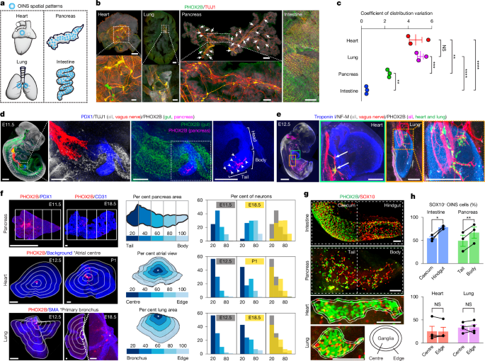
Results presented in Fig. 1c. PHOX2B-labelled OINS cells from the E18.5 cardiac atria, lungs, splenic lobe of the pancreas (tail and body), and small intestine were segmented as described in ‘Cell segmentation’. z-Projected images were generated to obtain organ outlines in Fiji, and the xy coordinates of PHOX2B cells were used for analysis. In MATLAB, we partitioned the organ areas into 200 µm × 200 µm grids and quantified neuron counts per grid. We then computed the standard deviation and mean of neuron counts across grids covering the organ area and calculated the coefficient of variation as their ratio. Left and right lung lobes were analysed separately and averaged.

Visualization of vagal nerves and OINS entry in embryonic images

Results presented in Fig. 1d,e. Immunolabelled vagal nerves in E11.5 and E12.5 embryos were manually outlined as ROIs encompassing the nerve structures throughout the z-stack. These ROIs were used to separate the image data into two stacks containing either the vagal nerve fluorescence or the remaining nerve fluorescence. The two image stacks were then merged as separate channels and visualized in different colours (red for vagal nerves, grey for other nerves). The same approach was applied to PHOX2B-immunolabelled cells in the pancreas, heart and lungs. PHOX2B cells within the organs were manually segmented to generate ROIs used to create separate stacks containing either fluorescence signals from cells inside or outside the organs, which were then visualized in different colours. The pancreas was visualized by PDX1 immunofluorescence, the heart by Troponin I immunofluorescence, and the lungs by autofluorescence detected in the Troponin I channel.

OINS distribution patterns during development

Results presented in Fig. 1f and Extended Data Fig. 1f–k. For the pancreas, heart, and lungs, PHOX2B-labelled cells were segmented at each developmental stage as described in ‘Cell segmentation’. z-Projected images were generated in Fiji to obtain organ outlines, and the xy coordinates of PHOX2B cells were used for analysis. For the pancreas, the splenic lobe (tail and body) was analysed. Two points were manually selected at opposite edges of the pancreas, one at the tail and one at the body. Samples were oriented horizontally along the tail–body axis using the two edge points. The pancreatic area was divided into five segments from tail to body (20%, 40%, 60%, 80% and 100%), and PHOX2B cell counts were obtained for each segment. The fraction of neuron counts per segment to the total neuron count was calculated. For the hearts, four atrial landmarks (anterior edge, posterior edge and right and left junctions between the atrial dome and appendages) were manually selected. The centroid of these landmarks was computed and used as the atrial centre. For the lungs, the right lobes were analysed, and a point at the primary bronchial trunk was manually selected as primary bronchus. From the defined reference point (atrial centre for the heart; primary bronchus for the lungs) towards the organ outline, five contour zones (20%, 40%, 60%, 80% and 100% of the organ area) were generated following the organ shape. PHOX2B cell counts were obtained for each zone, and the fraction of neuron counts per zone to the total neuron count was calculated.

Wavefront analysis

Results presented in Fig. 1g,h. Image stacks from E12.5 samples (intestine, pancreas, hearts and lungs) immunolabelled for SOX10 and PHOX2B were z-projected in Fiji. On the z-projected images, SOX10 and PHOX2B fluorescence signals were segmented by applying binary thresholds to generate ROIs encompassing the respective fluorescence areas. Organ outlines for the intestine and pancreas, and ganglion outlines for the hearts and lungs were also obtained. The ROIs were imported into MATLAB and converted into polygonal regions. Areas containing SOX10 or PHOX2B signals were combined to define the total neuronal area. The intestine and pancreas were each divided into two halves along their longitudinal axis (cecum and hindgut for intestine; tail and body for pancreas). For each half, the SOX10⁺ fraction was calculated by dividing the SOX10⁺ signal area by the total neuronal area. For the hearts and lungs, each ganglion was divided into centre and edge zones, with the edge zone defined as a peripheral band along the ganglion boundary. For each zone, the SOX10⁺ fraction was calculated by dividing the SOX10⁺ signal area by the total neuronal area.

Correlation analysis between NPCs and OINS distribution variability

PHOX2B, SOX10 and Ki67-labelled cells were manually segmented in Fiji throughout z-stack images. Among PHOX2B⁺Ki67⁺ cells, the SOX10-negative fraction was calculated as the number of SOX10-negative cells divided by the total number of PHOX2B⁺Ki67⁺ cells, representing the proportion of NPCs among proliferating cells. The correlation between NPCs (Fig. 2b) and OINS distribution variability (Fig. 1c) was assessed by linear regression (R²) in GraphPad Prism, as shown in Fig. 2l.

scRNA-seq and data analysis

Cell dissociation and sequencing

For scRNA-seq of OINS cells, the heart, lungs, pancreas and intestines were dissected from Wnt1-cre; lox-tdTomato, Phox2b-Flpo;frt-tdTomato, or Baf53b-cre; lox-L10GFP mice as indicated at E12.5, E14.5, E16.5, E18.5 and P56 in ice-cold Leibovitz’s L-15 Medium (Gibco). For the hearts and lungs, fluorescently labelled OINS regions were isolated by microdissection under a Leica M205FCA fluorescence stereomicroscope. For experiments comparing heart^near and heart^far regions, atrial areas containing Wnt1-cre; lox-L10GFP labelled ICNS cells were dissected to separate from the atrial areas lacking ICNS. Dissected tissues were cut into 1–3 mm² pieces and incubated in 0.25% trypsin-EDTA (Gibco) at 37 °C for 10 min (E12.5, E14.5) or 20 min (E16.5, E18.5, P56) with shaking. After washing with L-15 medium containing 10% fetal bovine serum (L15/FBS), tissues were incubated in 2 mg ml⁻¹ Collagenase A (Sigma-Aldrich) and 2 mg ml⁻¹ of Dispase II (Sigma-Aldrich) in 1× HBSS at 37 °C for 30 min (E12.5, E14.5) or 40 min (E16.5, E18.5, P56) with shaking. After washing with L15/FBS, cells were separated into single cells by trituration using three fire-polished Pasteur pipettes of decreasing diameter. Mature ICNS neurons isolated from Baf53b-cre; lox-L10GFP hearts at E18.5 and P56 were further purified using 30% and 60% Percoll density gradients. The cell suspension was filtered through a 40-μm cell strainer (Corning). All centrifugation steps were performed at 200g at 4 °C. After the final centrifugation, the cell pellet was resuspended in 1× HBSS containing 0.04% BSA. Fluorescently labelled cells were sorted on a BD FACSAria cell sorter with BD FACSDiva v9.4 at Yale Flow Cytometry Facility and collected in ice-cold 1× HBSS containing 0.04% BSA (Supplementary Fig. 1). Single-cell cDNA libraries were prepared using the Chromium Single Cell 3′ V3 reagent kit and sequenced using an Illumina NovaSeq 6000 S4 sequencer at Yale Center for Genomic Analysis, generating 300 million reads per sample at a depth of 20,000−300,000 reads per cell.

Basic scRNA-seq data processing and quality control

Raw sequencing data were aligned to the mm10-2020-A mouse genome reference using Cell Ranger software v.7.1.0 (10x Genomics). Cells were filtered based on standard quality control metrics (nFeature_RNA 200–20,000 and percent.mito <10%). Unsupervised clustering, data integration, differentially expressed gene (DEG) analysis and UMAP visualization were performed following the R package Seurat v.4.3.0⁵³ using Rstudio (2021.09.2 build 382). Integration of E14.5 scRNA-seq datasets of ICNS, intrapulmonary neurons, intrapancreatic neurons and ENS was performed using the portal integration method (see ‘Portal integration of OINSs from the heart, lungs, pancreas and intestines’). Cell cycle phase assignment for E12.5, E14.5 and E16.5 ICNS integrated datasets was performed using the CellCycleScoring function. DEGs were identified using the FindMarkers function with the bimodal likelihood-ratio test. GO enrichment analysis of DEGs was performed with the Gene Ontology Resource GO Enrichment Analysis tool^54,55 (http://geneontology.org). The AnimalTFDB 3.0 database⁵⁶ was used for identifying mouse transcription factors. For each OINS, the following mouse strains, numbers of mice and Phox2b⁺ cell counts that passed quality control were included in this study: heart, E12.5 (Wnt1-cre; lox-tdTomato, 35 embryos, 1124 cells), E14.5 (Wnt1-cre; lox-tdTomato, 14 embryos, 4,745 cells), E16.5 (Wnt1-cre; lox-tdTomato, 15 embryos, 4,615 cells), E18.5 (Baf53b-cre; lox-L10GFP, 7 embryos, 547 cells); lung, E14.5 (Phox2b-Flpo; frt-tdTomato, 12 embryos, 1,796 cells); pancreas, E14.5 (Phox2b-Flpo; frt-tdTomato, 10 embryos, 2,973 cells); intestine, E14.5 (Phox2b-Flpo; frt-tdTomato, 7 embryos, 4,395 cells).

Cell motility score calculation

The AddModuleScore⁵⁷ function in Seurat was used to calculate a cell motility score using 379 genes overlapping between those annotated under the GO term ‘cell motility’ (GO:0048870) and the top 2,000 variable genes from the integrated E12.5/E14.5/E16.5 ICNS dataset (Fig. 2k). For each cell, the expression levels of these genes were averaged to generate the final cell motility score.

Portal integration of OINSs from the heart, lungs, pancreas and intestines

We utilized Portal (v1.0.4)⁵⁸ to integrate the E14.5 scRNA-seq datasets of ICNS, intrapulmonary neurons, intrapancreatic neurons and ENS (Fig. 3b-j). For each dataset, function portal.utils.preprocess_datasets implemented in the Portal pipeline was employed to identify the top 2,000 highly variable genes. The gene expression matrices of these shared highly variable genes across the four datasets were then used as inputs to the Portal integration function portal.utils.integrate_datasets. Through an adversarial learning mechanism, Portal projected the gene expression profiles of cells from multiple datasets into a shared 20-dimensional space, eliminating batch effects while preserving biological variations from each dataset. The harmonized cell representations in this 20-dimensional space were subsequently used for unsupervised cell clustering and UMAP visualization following the Seurat pipeline, and Slingshot trajectory inference.

RNA velocity inference

We inferred the cell state transitions of ICNS cells at E14.5 using RNA velocity (Extended Data Fig. 3b). Starting from the CellRanger output, we used the velocyto run10x function⁵⁹ to extract spliced and unspliced read count matrices. Then we performed the following necessary data processing steps. We selected the top 2,000 highly variable genes based on dispersion to construct the PCA space. We then computed cell-wise moments for RNA velocity estimation using each cell’s 30 nearest neighbours, determined from the top 30 PCs. Using the processed data, we applied veloVI (v0.3.1)⁶⁰ using the function velovi.VELOVI. Finally, we visualized the RNA velocity results using scvelo.pl.velocity_embedding.

Monocle trajectory inference

Monocle 3⁶¹ v1.3.1 was used to infer the trajectory of the integrated E12.5, E14.5 and E16.5 ICNS datasets. The starting point of the trajectory was determined by 50 precursor-state cells with the highest Sox10 expression. The cells within the precursor-to-neuroblast branch (Extended Data Fig. 3c) were selected by the choose_cells function. To isolate genes that vary significantly along this branch, the graph_test function was applied with a threshold of q-value < 0.01. We computed the gene dynamics over pseudotime to generate a time series of gene expression levels. Then we applied a threshold to retain genes showing expression changes greater than 0.3 across pseudotime. We next performed hierarchical clustering and classified these 2,734 highly variable genes based on their expression patterns over pseudotime using the cutree function with a cluster number set at 13 (k = 13). Within the initial 13 clusters, groups sharing similar expression patterns were further combined, resulting in the final 6 distinct modules (Extended Data Fig. 3d,e). The GO analysis of the module genes was performed using the Gene Ontology Resource GO Enrichment Analysis tool^54,55 (http://geneontology.org).

Trajectory and pseudotime inference using Slingshot

We used Slingshot (v2.6.0)⁶² to infer the trajectory and pseudotime of the integrated E14.5 scRNA-seq datasets of ICNS, intrapulmonary neurons, intrapancreatic neurons and ENS (Fig. 3d–j). Before applying Slingshot, we performed unsupervised cell clustering on the integrated cell representations from Portal using functions FindNeighbors and FindClusters implemented in Seurat, identifying eight distinct Seurat clusters. These clusters were then assigned to three cell states: precursors, neuroblasts and neurons. The slingshot function was applied to identify the branching structure of OINSs by ordering these cell clusters, with the precursor population defined as the beginning and the neuron population as the end of the trajectory. Finally, within the same function, Slingshot inferred the pseudotime of cells along each branch of the trajectory.

CellChat

To quantify interactions between organ cells and OINSs, Seurat objects of organ cells were pairwise merged with the corresponding E14.5 OINS scRNA-seq datasets generated in this study (4,554 organ cells and 1,796 OINS cells per pair). Organ datasets were our E14.5 heart^near and intestinal scRNA-seq datasets (with ENS cells removed by fluorescence-activated cell sorting (FACS)) and from published lung and pancreas datasets (E15.5 lung⁶³; E14.5 pancreas⁶⁴). For comparing interaction strengths between the heart^near or heart^far regions with ICNS, we pairwise merged the heart^near or heart^far to the ICNS Seurat objects using 3,093 cells from each dataset. As a reference, 3,093 fibroblasts and 3,093 cardiomyocytes^65,66 were randomly sampled from the heart^near and heart^far datasets and merged as a control pair. With the CellChat package v1.6.1⁶⁷, we transformed the merged Seurat objects into the CellChat objects using the normalized data matrix stored within the ‘RNA’ assay. We incorporated the CellChat object with the CellChatDB.mouse database, identified overexpressed genes and interactions using identifyOverExpressedGenes and identifyOverExpressedInteractions, and computed their communication probabilities using computeCommunProb (population.size = FALSE, type = “truncatedMean”, trim = 0.05) and filterCommunication (min.cells = 100). Finally, we obtained the communication probabilities of individual ligand–receptor pairs with P value < 0.05 using subsetCommunication. From the resulting data frame, organ–to–neuron interactions were defined as ligand–receptor pairs with organ cells as ‘source’ and neurons as ‘target’. For reference fibroblast–cardiomyocyte interactions, ligand–receptor pairs were extracted in both directions. The CellChatDB.mouse database includes three signalling annotations: secreted signalling, cell–cell contact and ECM–receptor. For organ–to–neuron interactions (Fig. 4j), we summed the communication probabilities (prob) of ligand–receptor pairs annotated as ECM–receptor. For heart^near–ICNS and heart^far–ICNS comparisons, probabilities were summed across all three signalling categories, as was done for the fibroblast–cardiomyocyte reference interactions (Extended Data Fig. 12c).

Cross-organ similarity analysis along the Slingshot-inferred trajectory

To evaluate how E14.5 OINSs from each organ resemble those from the other organs along the Singshot inferred pseudotime trajectory (Extended Data Fig. 6e), we pre-processed the raw count matrices of OINSs from the four organs using the functions sc.pp.normalize_total, sc.pp.log1p and sc.pp.scale following the Scanpy pipeline. Next, we performed a joint PCA analysis on the processed data and identified the top 50 principal components. For each cell, we identified its k = 200 nearest neighbours from each of the other three organs. We then computed cosine similarities between the top 50 principal components of each cell and the averaged top 50 principal components of its k nearest neighbours from each of the other organs, which yielded three cosine similarity scores per cell. The mean of these three scores quantified the overall cross-organ similarity for that cell. We generated a scatter plot illustrating individual cells with the x axis as pseudotime and the y axis as the mean cosine similarity to visualize how transcriptomic similarity between OINSs and different organs changes across differentiation. A fourth-order polynomial regression curve was fitted to capture the trend for each organ.

Estimating cell fate transition probabilities along the Slingshot-inferred trajectory

We used Portal to integrate E14.5 scRNA-seq OINS datasets from the heart, lungs, pancreas and intestine and generated harmonized low-dimensional representations of cells across the four datasets. These representations were projected back into gene expression space to derive integrated, log-normalized expression profiles, which served as input for cell fate transition analysis. For this analysis (Fig. 3i), we applied moscot.time from the moscot framework (v0.4.2)⁶⁸, which uses optimal transport to probabilistically link cells across developmental time points. To model cell state transitions along the differentiation trajectory of our E14.5 OINS datasets, we divided the Slingshot-inferred trajectory into overlapping time stages based on pseudotime. Each time stage spanned a pseudotime interval of 3, with adjacent stages offset by 0.5 to allow for overlap. For the trajectory ranging from pseudotime zero to the end, the resulting stages included time windows such as 0.0−3.0, 0.5−3.5, 1.0−4.0, and so on. Using these time windows, we applied moscot.time to infer transitions between each pair of non-overlapping adjacent stages—for example, linking the 0.0–3.0 window (early) to the 3.0–6.0 window (late), or 0.5–3.5 to 3.5–6.5. In each application of moscot.time, we considered two organs (for example, organ A and organ B) and computed a transition probability matrix \(P\in {R}^{{N}_{{\rm{early}}}\times {N}_{{\rm{late}}}}\), where \({N}_{{\rm{early}}}\) and \({N}_{{\rm{late}}}\) are the numbers of cells in the early and late time windows, respectively. Each entry \({P}_{{ij}}\) represents the probability of cell \(i\) in the early-stage transitioning to cell \(j\) in the late stage. To summarize these cell-level transition probabilities at the organ level, we calculated, for each early-stage cell \(i\), the probability of transitioning into late-stage cells from organ A and organ B, respectively. These organ-level probabilities are defined as:

where \({C}_{{\rm{late}},{\rm{organ}}{\rm{A}}}\) and \({C}_{{\rm{late}},{\rm{organ}}{\rm{B}}}\) denote the sets of late-stage cells originating from organ A and organ B, respectively. If a given early-stage cell \(i\) appeared in multiple applications of moscot.time (due to overlapping time windows), we computed its final organ-level transition probabilities by averaging the values obtained from all relevant applications. For instance, a cell with pseudotime 0.6 appeared in both the 0.0–3.0 to 3.5–6.5 and 0.5–3.5 to 3.5–6.5 transitions. Its final probabilities of transitioning to organ A and organ B, denoted \({\widetilde{p}}_{i}^{\mathrm{organ}\,A}\) and \({\widetilde{p}}_{i}^{\mathrm{organ}\,B}\), were computed by averaging the corresponding values \({p}_{i}^{\mathrm{organ}\,A}\) and \({p}_{i}^{\mathrm{organ}\,B}\) respectively, across those applications. Finally, to examine the temporal dynamics and uncertainty of organ-level transition probabilities, we analysed each organ pair (organ A and organ B) separately. For each cell from organ A, we plotted its pseudotime values (x axis) against its transition probability \({\widetilde{p}}_{i}^{\mathrm{organ}\,A}\) to organ A (y axis). Similarly, for cells from organ B, we plotted their pseudotime (x axis) against their transition probability \({\widetilde{p}}_{i}^{\mathrm{organ}\,A}\) to organ A (y axis). To describe and compare these two trends, we used the geom_smooth function in R to fit smooth curves between pseudotime and transition probabilities (mean ± 95 % confidence interval) for each of the two organs, thereby revealing their dynamics of cell fate transitions along the trajectory.

Quantification of pairwise OINS similarity score

We assessed similarities among OINSs across organs (Fig. 3j) using two approaches. The first compared how OINS cells from each organ were distributed across the four trajectory branches identified by Slingshot. For each branch, we computed the proportion of OINS cells from each organ, and pairwise organ differences in branch patterns were quantified by calculating the Euclidean distance between the corresponding organ-specific proportion vectors. The second approach quantified how much the OINS fate transition trajectory of one organ diverged from that of another. For each organ pair, we used the two previously fitted smooth curves representing the dynamics of cell fate transitions along the trajectory (see ‘Estimating cell fate transition probabilities along the Slingshot-inferred trajectory’) and measured the pairwise difference as the area between the two fitted curves. Between-organ difference values from the two approaches were linearly rescaled to a range of 0–1, where 0 indicates the greatest difference and 1 represents identical OINS patterns between the 2 organs.

Integration of maturing ENS and ICNS neurons

Published E15.5, E18.5 and P21 ENS scRNA-seq datasets¹⁸ were used for ENS/ICNS integration (Fig. 3k). High-quality neuroblasts and neurons were retained using stringent filters: for E15.5/E18.5, nCount_RNA 5,000–30,000, nFeature_RNA 2,500–6,000, percent.mito <5%, and Plp1 < 0.1; for P21, nCount_RNA 5,000–50,000, nFeature_RNA 2,500–7,500, percent.mito <10%, and Plp1 < 0.1. A total of 1,400 E15.5, 900 E18.5, and 900 P21 cells were randomly selected for downstream analyses. For ICNS, our E14.5, E16.5 (Wnt1-cre; lox-tdTomato) and E18.5, P56¹⁰ (Baf53b-cre; lox-L10GFP) scRNA-seq datasets were used. High-quality neuroblasts and neurons were retained using stringent filters: for E14.5, nCount_RNA 10,000–30,000, nFeature_RNA 3,000–6,000, percent.mito <5%, Phox2b > 0, Mki67 < 0.1, and Plp1 < 0.1; for E16.5, nCount_RNA 5,000–30,000, nFeature_RNA 2,000–7,000, percent.mito <5%, Mki67 < 0.1, Phox2b > 0, and Plp1 < 0.1; for E18.5/P56, nCount_RNA 30,000–100,000, nFeature_RNA 6,000–10,000, percent.mito <5%, Plp1 < 0.1, and Phox2b > 0. To best capture the ICNS trajectory towards mature neurons, the neuroblast and neuron populations were balanced in E16.5, and the Npy and Ddah1 populations were balanced in P56. A total of 900 E14.5, 250 E16.5, 250 E18.5, and 500 P56 cells were randomly selected for downstream analyses. Integration followed the standard Seurat workflow, with the integration order set so that ICNS datasets were mapped to ENS datasets. Neuron types were identified as described before^10,18. We quantified similarity among cell populations using cosine similarity. For each cell, we extracted the top 50 principal components from the integrated gene expression matrix. We then computed the average principal component vector across cells within each population. Pairwise similarities between cell populations were finally assessed by calculating the cosine similarity between their averaged principal component vectors.

Spatial dynamics of ICNS cells

Geometric transformation of 3D heart images

For data presented in Fig. 5i and Extended Data Figs. 14 and 15a–h, heart samples (E12.5–P1) were imaged as intact three-dimensional structures from the atrial view using a Leica SP8 confocal microscope equipped with a 16× immersion objective as described in ‘Whole-embryo or organ clearing and immunofluorescence staining’. PHOX2B-labelled ICNS cells were segmented as described in ‘Cell segmentation’. Four atrial landmarks (anterior edge, posterior edge and right and left junctions between the atrial dome and appendages) were manually selected. Three ICNS reference planes were defined using these landmarks as follows. First, a best-fit atrial plane (plane-z) was defined by singular-value decomposition of the landmark matrix after centring the landmarks’ coordinates on their mean and taking the third right-singular vector as the plane’s normal. This approach yields a plane that best fits all landmarks. Second, landmarks were projected onto plane-z and a secondary atrial midline plane (plane-y) was defined through the midpoint of the projected anterior and posterior landmarks, oriented perpendicular to the anterior–posterior axis. Finally, a third orthogonal plane (plane-x) was constructed from the cross-product of plane-z and plane-y and positioned also at the same midpoint used for plane-y. For each ICNS cell, the perpendicular distances to the three reference planes (plane-x, plane-y and plane-z) were calculated using the dot product between the normalized plane vector and the neuron’s xyz coordinates. These distances defined the transformed ICNS coordinates, allowing all samples to be compared in the same orientation. As ICNS cells were predominantly distributed on plane-z, the transformed ICNS xy coordinates were used for spatial distribution analysis. A two-dimensional area (2,000 µm × 2,000 µm) encompassing all transformed ICNS cells was partitioned into 50 × 50 µm grids. The number of ICNS cells within each grid was counted. The resulting 2D-transformed ICNS count maps were used for subsequent spatial quantifications.

To visualize spatial distribution heat maps of ICNS (Fig. 5i), 2D-transformed ICNS count maps across samples were averaged and plotted as filled contour plots for each developmental stage. To assess the landing sites of ICNS (Extended Data Fig. 14g,h), individual ICNS cell coordinates from E12.5 cardiac atria immunolabelled for PHOX2B were manually identified throughout the image stacks and their xy coordinates were imported to MATLAB. A neighbour connectivity graph was constructed based on pairwise Euclidean distances between all ICNS cells. Cells with intercellular distances ≤25 µm were connected into groups. Each group was defined as an individual landing site. Groups containing ≤10 cells were considered small aggregates and were merged with the nearest landing site. The resulting merged groups represented the final set of landing sites. To compare ICNS spatial distributions across animals and developmental stages (Extended Data Fig. 15b), each sample’s 2D-transformed ICNS count map was normalized to the distance between the projected anterior and posterior landmarks. The normalized 2 × 2 area was partitioned into 0.1 × 0.1 grids. For each sample, ICNS cell counts per grid were divided by the total number of ICNS cells to generate a probability map. The mean probability map for each developmental stage was computed as the grid-wise mean across samples within that stage. For each sample, deviations from the stage mean were calculated by subtracting the mean probability map from the sample’s probability map grid by grid, squaring the differences, and summing across all grids. The resulting summed-squared deviation provided a measure of how much each sample’s ICNS spatial distribution differed from its age average. To quantify ICNS cell density and total ICNS cluster area (Extended Data Fig. 15d,e), a grid containing at least three ICNS cells was classified as an ICNS-containing grid. Total ICNS cluster area was calculated as the number of ICNS-containing grids multiplied by 2,500 μm². ICNS cell density was calculated by dividing the cell number in ICNS-containing grids by the total ICNS cluster area. For each ICNS cell, the mean distance to its ten nearest neighbours was calculated, and the average of these values per animal was plotted as individual data points in Extended Data Fig. 15f. To identify disconnected ICNS clusters (Extended Data Fig. 15g), grids containing at least three cells or more than 20% of the maximum cell count per grid were defined as ICNS-positive. Adjoining ICNS-positive grids connected horizontally, vertically, or diagonally were grouped as a cluster. Clusters containing grids with more than 50% of the maximum cell count per grid were identified as final ICNS clusters. To assess the inner area of the ICNS ring (Extended Data Fig. 15h), the 2D-transformed ICNS count maps were plotted as contour maps. The inner region enclosed by ICNS contours was manually outlined in Fiji, and the enclosed area was measured to determine the inner area of the ICNS ring.

Analysing ICNS organization in Itga1 and Lox knockout mice

Atrial regions of wild-type and knockout mice (P5 for Itga1 knockout; P0 for Lox knockout) were dissected, cleared using CUBIC and immunolabelled with anti-PHOX2B (AF4940, R&D Systems) and anti-beta III tubulin (TUJ1, ab18207, Abcam) as described in ‘Whole-embryo or organ clearing and immunofluorescence staining’. The atria were flattened along the superior axis and imaged in a custom-made metal box on a Leica SP8 confocal microscope with a 10× objective using Leica Application Suite X software (v3.5.7.23225). Individual PHOX2B-labelled neurons and their coordinates were manually segmented in Fiji from the stack images. For each sample, the ICNS ring was manually identified along the thick TUJ1 fibres connecting major ICNS ganglia, and the xy coordinates of the ring centre were determined. The anterior ICNS cluster located adjacent to the superior vena cava was outlined manually, and its centre coordinates were obtained. Because all images were acquired from the superior view of the atria in similar orientations, each sample was aligned by rotating along the axis defined by the anterior ICNS cluster and the ICNS ring centre, and then re-centred to its ring centre. Aligned samples were overlaid and colour-coded to visualize ICNS distributions in wild-type and knockout hearts. For each sample, a 6,000 µm × 6,000 µm area encompassing all ICNS neurons was partitioned into 200 µm × 200 µm grids, and the neuron count within each grid was quantified. For wild-type and knockout groups, the standard deviation of neuron counts in each grid across animals was calculated. Higher standard deviations suggest more variable ICNS structures.

For identifying loss of neurons in specific ICNS clusters in Itga1-knockout mice, G1–G4 ICNS clusters (Fig. 4l) of wild-type and knockout hearts were manually defined by grouping cells according to the sectors of the polar plots. In GraphPad Prism, one large outlier in G2 cluster of wild type and one small outlier in G1 cluster of knockout were identified using the ROUT method (Q = 1%) and excluded from statistical comparisons. For each cluster, the number of ICNS cells was normalized to the wild-type mean, and the normalized neuron numbers between wild type and knockout were compared using multiple unpaired t-test with the Holm–Šídák correction.

For identifying changes in ganglionic structures in Lox knockout mice, neuron clusters were defined based on neighbour connectivity, by which neurons with Euclidean distances ≤ 25 µm were considered neighbours belonging to the same cluster. Major ganglia were defined as clusters containing more than 50 neurons, and mini clusters were defined as those with ≤ 50 neurons.

Ascl1
^creER-tdT-mediated lineage tracing

Ascl1-creERT2 mice were crossed with lox-tdTomato mice. On E12.5, a single dose of 4-hydroxytamoxifen (Sigma-Aldrich, H6278) was administered to pregnant mice by intraperitoneal injection at 50 mg kg⁻¹. After 8 days, the hearts, lungs, pancreas and intestines from Ascl1^creER-tdT mice were dissected and co-immunolabelled with RFP and PHOX2B antibodies. The number of PHOX2B cells and the fraction expressing tdTomato were quantified for each organ and compared using Holm–Šídák multiple-comparisons test following ordinary one-way ANOVA. To estimate changes in the number of Ascl1⁺ precursors in the ICNS (Fig. 2j), we calculated the number of Ascl1⁺ cells at each stage as follows. The Ascl1⁺ cell number by birth was derived by multiplying the mean E18.5 ICNS cell count by the proportion of Ascl1^creER-tdT cells in the heart as shown in Fig. 2i. The E12.5 Ascl1⁺ cell number was estimated by multiplying the total E12.5 ICNS cell count by the fraction of Ascl1⁺ cells identified in the E12.5 scRNA-seq ICNS dataset. For quantification of the proportion of ICNS neurons among Ascl1-labelled cells in the heart, the number of tdTomato⁺ cells and the fraction expressing PHOX2B immunofluorescence within the ICNS ganglia were counted.

BrdU assay

BrdU at 100 mg kg⁻¹ was intraperitoneally injected to pregnant mice carrying E14.5 Wnt1-cre; lox-tdTomato embryos. One hour after injection, the pregnant mice were euthanized and embryos were collected. Hearts were dissected and fixed in 4% ice-cold PFA overnight at 4 °C, cryoprotected in 30% sucrose PBS solution for two days at 4 °C, embedded in OCT, and stored at −80 °C until cryosectioning. Sections (10 μm) were cut using a cryostat (Thermo Fisher Scientific) and mounted onto Superfrost Plus slides (Thermo Fisher Scientific). Sections were incubated with 1 M HCl for 1 h, neutralized with 0.1 M Sodium Borate (pH 8.5) for 10 min, washed, permeabilized (0.1% Triton X-100 in PBS), blocked (5% normal donkey serum, 0.1% Triton X-100 in PBS) and incubated with anti-BrdU (ab6326, Abcam) and anti-PHOX2B (AF4940, R&D Systems) diluted in blocking buffer at 4 °C overnight. After washing, slides were incubated with donkey anti-goat-488 (705-545-147, Jackson ImmunoResearch) and donkey anti-rat-647 (712-605-150, Jackson ImmunoResearch) diluted in blocking buffer for 2 h at room temperature. After incubation, the samples were washed and mounted with ProLong Diamond Antifade Mountant with DAPI (Thermo Fisher Scientific). Images were acquired using a 20× objective (HC PL APO 20×/0.75 CS2) on a Leica SP8 confocal microscope.

Spatial transcriptomics with 10x Visium

Hearts from E14.5 Wnt1-cre; lox-Sun1-GFP mice were acutely dissected and freshly frozen in OCT. Cryosections (10 μm) were cut using a cryostat (Thermo Fisher Scientific) and mounted onto the 10x Visium Spatial Gene Expression Slide. Tissue sections were imaged on a Leica SP8 confocal microscope with a 16× objective to obtain tissue morphology and locate ICNS ganglia. Sequencing libraries were prepared following the manufacturer’s protocol (10x Visium) and sequenced using an Illumina NovaSeq S4 sequencer at Yale Center for Genomic Analysis. Raw FASTQ files and corresponding confocal images were processed by the Space Ranger software 2.0.0 (10x Genomics). We pre-processed the 10x Visium dataset using log-normalization^69,70. Gene expression values for each spot were normalized to the total number of transcripts and multiplied by a scaling factor of 10,000. The normalized dataset was then transformed to log scale using log1p. The log-normalization process was performed using the Python package Scanpy 1.8.2⁷⁰. Following this standard data pre-processing, we visualized gene expression levels within spots on a high-resolution histology image to examine spatial distributions of genes. The high-resolution image is a down-sampled version of the original full-resolution histology image, typically generated by the Space Ranger pipeline. It has 2,000 pixels in its largest dimension. To map spatial spots onto the high-resolution image, we utilized a text file that describes spot coordinates and a JSON file that describes image properties. The text file and the JSON files are outputs from the Space Ranger pipeline. The text file contains the pixel coordinates of spot centres on the full-resolution image, while the JSON file includes the spot diameter in pixels on the full-resolution image, as well as a scaling factor that transforms pixel positions from the original full-resolution image to the high-resolution image. Additionally, we visualized region of interest (ROIs) for the ICNS on the high-resolution histology image. We circled and saved ROIs using the Fiji software and loaded ROIs into Python using Python module read-roi (v1.6.0) for the joint visualization of ROIs, gene expression levels within spots, and the high-resolution histology image.

RNAscope HiPlex assay

RNAscope HiPlex assays were performed following the manufacturer’s instructions (Advanced Cell Diagnostics) as previously described⁷¹. OINS regions of E14.5 heart, E16.5 heart and E16.5 intestines of Wnt1-cre; lox-Sun1-GFP mice were dissected and freshly frozen in OCT. Cryosections (10 μm) were cut using a cryostat (Thermo Fisher Scientific), mounted on Superfrost Plus slides (Thermo Fisher Scientific), and stored at −80 °C until use. Slides were fixed with 4% PFA in RNase-free PBS for 60 min at room temperature, dehydrated through 50%, 70% and 100% ethanol, digested with Protease IV for 30 min at room temperature and treated with HiplexUp reagent to quench endogenous fluorescence. Sections were hybridized with the following probes for 2 h at 40 °C: Hoxa5 (T4), Phox2b (T6), Isl1 (T7), Fn1 (T8, round 1), Lox (T9), Myl4 (T10), Pecam1 (T12) and Wt1 (T8, round 2). After hybridization, sections were treated with HiPlex Amp followed by HiPlex Fluoro solutions, and imaged in 4× SSC on a Leica SP8 confocal microscope with a 16× immersion objective. Fluorophores were cleaved with 10% cleaving solution (ACD, 324130) between imaging rounds, and probes were removed using HiPlexUp reagent before the next hybridization. For Extended Data Fig. 6d, anti-HuC/HuD (Elavl3; A-21271, Invitrogen) immunolabelling was performed to visualize all neurons after probes were removed. For Fig. 5f, distances between ICNS and cardiac cell type fluorescence signals were measured in six independent E16.5 sections. For each section, ten straight-line distances were drawn between the nearest ICNS (Isl1) signal boundary and the boundary of the indicated cardiac cell type signal (Fn1, Myl4 or Wt1), yielding 60 measurements in total. Each dot in Fig. 5f represents one measurement.

Label-free quantitative mass spectrometry analysis

E14.5 hearts from Wnt1-cre; lox-L10GFP mice were dissected on ice under a Leica M205FCA fluorescence stereomicroscope to separate the atrial region that contained fluorescently labelled ICNS cells (heart^near) from the adjacent region lacking them (heart^far). Dissected tissues were collected into 1.5-ml tubes, snap-frozen with liquid nitrogen, and stored at −80 °C. Each sample comprised approximately 1 mm³ of tissues pooled from four embryos. Samples were subjected to label-free quantitative mass spectrometry analysis at the Keck Biotechnology Resource Laboratory at Yale University. P values were calculated using two-sided two-way ANOVA, assuming that the conditions are independent and applying the statistical test that assumes the means of the conditions are equal. No adjustments were made for multiple comparisons.

Simulation of ICNS organization formation

ICNS organization during cardiac cell proliferation (Extended Data Fig. 15j) was simulated in MATLAB (R2023a, MathWorks). Cardiac and ICNS cells were positioned in elliptical regions and their initial cell density was 0.01. Cardiac and ICNS proliferation rates were 0.5 and 0.01 per cycle, respectively. Dividing cells were randomly selected, and each generated one daughter cell that moved two units away from its parent in a random direction. After each proliferation cycle \(i\), cells migrated for \(50+10i\) steps. Cells with nearest-neighbour distances <10 units moved away along the local density gradient calculated using inverse-distance-squared weighting. Isolated ICNS cells (those with few nearby ICNS neighbours but many surrounding cardiac cells) moved towards the centroid of their 10 closest ICNS neighbours to mimic the clustering of ICNS. Cell positions of cardiac (green) and ICNS (red) populations were plotted after each step to form a stack image representing the simulation pseudotime.

ENS co-cultures with cardiac or intestinal cells for scRNA-seq

Cell dissociation and plating

Heart and intestines were dissected from E13.5 Phox2b-Flpo;frt-tdTomato embryos on ice under a Leica M205FCA fluorescence stereo microscope. Entire intestines were collected and hearts were trimmed to collect the atria. Cell dissociation was performed as described in ‘scRNA-seq and data analysis. To prevent contamination, all reagents for cell dissociation and FACS were supplemented with 100 U ml⁻¹ penicillin, 100 μg ml⁻¹ streptomycin and 100 μg ml⁻¹ Gentamicin. Dissociated cells were sorted on a BD FACSAria cell sorter at the Yale Flow Cytometry Facility (Supplementary Fig. 2a). tdTomato-positive and -negative cells were collected into separate tubes containing ice-cold cell culture medium, which contained Neurobasal Plus medium (Gibco A3582901) supplemented with 1% FBS (Thermo Scientific 10082147), 2 mM l-glutamine (Thermo Scientific 25030149), B-27 Plus Supplement (Gibco A3582801), 100 U ml⁻¹ penicillin, 100 μg ml⁻¹ streptomycin (Thermo Scientific 15140122), and 100 μg ml⁻¹ Gentamicin (Thermo Scientific 15710064). After FACS, cells were centrifuged at 200g for 10 min at 4 °C. For co-culture, 3,000 tdTomato⁺ ENS cells and 6,000 tdTomato-negative cardiac or intestinal cells were mixed and plated into 24-well plates pre-coated with a thin layer of Collagen I/Matrigel (Corning 356237) mixture that contains 0.5 mg ml⁻¹ of Matrigel and 33 μg ml⁻¹ Collagen I (Enzo Life Sciences ALX-522-440-0050) in cell culture medium. Cells were incubated at 37 °C in 5% CO₂ and co-cultured for 4–5 days.

Sequencing co-cultured ENS cells

After cell culture medium was removed, cells were incubated with 2 mg ml⁻¹ Collagenase A (Sigma-Aldrich) and 2 mg ml⁻¹ of Dispase II (Sigma-Aldrich) solutions at 37 °C for 10 min. The digested cells were collected into ice-cold 10% FBS L-15 medium (L15/FBS). This digestion was repeated 3-6 times until the coating layer was completely dissociated. Cells pooled from multiple wells were centrifuged at 200g at 4 °C for 10 min, washed three times with L15/FBS, and treated with Corning Cell Recovery solution (354253) on ice for 20 min to dissolve residual Matrigel. After two additional washes with L15/FBS, cells were gently triturated with a Pasteur pipet, filtered through a 40 μm cell strainer, washed three times, and resuspended in 1× HBSS, 0.04% BSA for scRNA-seq using the 10x Genomics platform.

scRNA-seq analysis of co-cultured ENS cells

Following the Seurat v.4.3.0⁵³ workflow, cells were filtered using standard quality control metrics (nFeature_RNA 200–20,000 and percent.mito <10%) and Phox2b⁺ clusters were identified from unsupervised clustering. For integration of datasets from ENS co-cultured with intestine (ENS^intestine) and with heart (ENS^heart), more stringent quality control thresholds (nFeature_RNA 2,500–20,000 and percent.mito <5%) were applied to the Phox2b⁺ population. Unsupervised clustering of the integrated dataset identified genetically distinct clusters and cell states were assigned based on cluster-specific gene expression. DEGs were identified within each cell state using FindMarkers (min.pct = 0.2, logfc.threshold = 0.25, test.use = ‘wilcox’) for the following comparisons: (1) precursors and neuroblasts: our E16.5 ICNS dataset compared with the published E15.5 ENS dataset¹⁸; (2) neurons: our E18.5 ICNS dataset compared with the published E18.5 ENS dataset¹⁸; and (3) co-culture neurons: ENS^heart compared with ENS^intestine. For each state in ENS^heart and ENS^intestine, expression levels of DEGs enriched in normal ICNS or ENS were quantified using the AddModuleScore⁵⁷ function and averaged per cell. Similarity scores were calculated by subtracting the mean ENS gene expression from the mean ICNS expression (Fig. 4c,d and Extended Data Fig. 11a,b). Positive scores indicate a more similar genetic programme to ICNS. Of the 663 genes upregulated in ENS^heart relative to ENS^intestine at the neuron state, 372 (56%) were also upregulated in ICNS relative to ENS neurons at E18.5. GO Enrichment Analysis tool^54,55 at Gene Ontology Resource was used to identify top GO terms in genes upregulated in both ENS^heart and E18.5 ICNS, and in both ENS^intestine and E18.5 ENS, at the neuron state. For each set, we visualized 106 genes in heat maps (Extended Data Fig. 10), including transcription factors and genes with the highest average log₂[fold change] within each GO term.

Imaging ENS differentiation under different co-culture conditions

Hearts, lungs, pancreas, and intestines were dissected from E13.5 Phox2b-Flpo;frt-tdTomato embryos on ice under a Leica M205FCA fluorescence stereomicroscope. Hearts and lungs were trimmed to collect the atria and pulmonary hilum, respectively. Mesenteries were removed from pancreas and intestines, and the entire organs were used for cell dissociation as described in ‘scRNA-seq and data analysis’. To prevent contamination, all reagents were supplemented with 100 U ml⁻¹ penicillin, 100 μg ml⁻¹ streptomycin, and 100 μg ml⁻¹ Gentamicin. Dissociated cells were sorted on a BD FACSAria cell sorter at the Yale Flow Cytometry Facility (Supplementary Fig. 2b). tdTomato-positive cells from intestines (ENS) and tdTomato-negative cells from all organs were collected into separate tubes containing ice-cold cell culture medium, which contained Neurobasal Plus Medium (Gibco A3582901) supplemented with 1% FBS (Thermo Scientific 10082147), 2 mM l-glutamine (Thermo Scientific 25030149), B-27 Plus Supplement (Gibco A3582801), 100 U ml⁻¹ penicillin, 100 μg ml⁻¹ streptomycin (Thermo Scientific 15140122), and 100 μg ml⁻¹ Gentamicin (Thermo Scientific 15710064).

For ENS co-cultures with organ cells, 5,000 tdTomato⁺ ENS cells and 5,000 tdTomato-negative organ cells were mixed and plated per well of 24-well plates coated with poly-l-ornithine (P4957, Sigma-Aldrich). For ENS co-cultures with conditioned organ medium, 5,000 tdTomato⁺ ENS cells and 5,000 tdTomato-negative organ cells were plated in separate wells. Media from organ-cell wells were refreshed and transferred daily to ENS-only wells. For ECM-supplemented cultures, 5,000 tdTomato⁺ ENS cells were plated per well coated with a mixture of fibronectin (3.5 μg per well, abcam ab92784), laminin (3.5 μg per well, Sigma-Aldrich L2020), collagens type I (25 μg per well, Sigma-Aldrich C3867), type II (7 μg per well, Sigma-Aldrich C9301), and type III (7 μg per well, Sigma-Aldrich CC054) in addition to poly-l-ornithine. All cultures were maintained at 37 °C in 5% CO₂ for 7 days. Cells were cultured in one well for each condition and were derived from three biologically independent embryos. Entire wells were imaged daily using a Leica DMi8 inverted confocal microscope with a 10× objective. For quantifying ENS differentiation, each well was divided into four quadrants, and individual cells were manually segmented; cells bearing neurites were counted as differentiated. Fraction of Differentiated ENS was quantified independently in each quadrant, and each quadrant represented one data point for statistical analysis.

Statistics and reproducibility

All statistical analyses were performed using GraphPad Prism 10. Data are presented as mean ± s.e.m., with sample size and specific statistical tests used indicated in the corresponding figure legends and Methods. All statistical tests were two-sided. Exact P values are reported in the figures. Statistical significance was defined as P < 0.05 (*P < 0.05; **P < 0.01; ***P < 0.001; ****P < 0.0001).

Experiments were repeated independently in multiple mice or samples with similar results. No statistical methods were used to predetermine sample size. Both sexes of mice were used. Randomization was not performed, since all experiments were performed with mice of the indicated age and genotype, and with mouse-derived cells under the indicated conditions. For the Lox-knockout and Itga1-knockout analyses, neuronal cell segmentation was performed in a blinded manner. Blinding was not applied in other experiments because group allocation was determined by predefined experimental variables such as age, organ type, or cell culture conditions.

The nature and number of replications are described in the figure legends or listed here: Fig. 1b: heart (n = 9 mice), lung (n = 4 mice), pancreas (n = 4 mice), intestine (n = 2 intestinal tissue pieces from one mouse); Fig. 1d (n = 3 mice); Fig. 1e (n = 3 mice); Fig. 1f and Extended Data Fig. 1f–k: mean histograms across all samples per age from pancreas (E11.5 n = 3; E12.5 n = 4; E14.5 n = 5; E16.5 n = 3; E18.5 n = 3 mice), heart (E12.5 n = 12; E13.5 n = 7; E14.5 n = 8; E16.5 n = 6; E18.5 n = 3; P1 n = 6 mice), lung (E12.5 n = 4; E14.5 n = 3; E16.5 n = 3; E18.5 n = 3 mice); Fig. 2a,b and Extended Data Fig. 2a: heart (n = 6 mice), lung (n = 4 mice), pancreas (n = 3 mice), intestine (n = 6 mice); Fig. 2h,i: heart (n = 4 mice), lung (n = 4 mice), pancreas (n = 4 mice), intestine (n = 4 mice); Fig. 2j (E12.5 n = 12 mice; by birth n = 3 mice); Fig. 4f,h,i and Extended Data Fig. 11c–e: cultured cells were derived from 3 independent embryos (see ‘Imaging ENS differentiation under different co-culture conditions’). Figure 5e (n = 20 sections from one mouse); Fig. 5h (n = 4 mice); Fig. 5i and Extended Data Fig. 15a–h (E12.5 n = 12; E13.5 n = 7; E14.5 n = 8; E16.5 n = 6; E18.5 n = 3; P1 n = 6 mice); Fig. 5j (n = 9 mice); Fig. 5k and Extended Data Fig. 12e,f (n = 20 sections from one mouse); Fig. 5l–o (WT n = 5; Lox KO n = 4 mice); Extended Data Fig. 1a–c (n = 3 mice); Extended Data Fig. 1d (n = 3 mice); Extended Data Fig. 1e (n = 4 mice); Extended Data Fig. 2b,c (n = 7 ganglia from one animal); Extended Data Fig. 2d (n = 2 mice); Extended Data Fig. 2e (n = 3 mice); Extended Data Fig. 2f (n = 4 mice); Extended Data Fig. 6d: heart (n = 20 sections from one animal), intestine (n = 7 sections from one animal); Extended Data Fig. 7b (n = 15 FACS experiments); Extended Data Fig. 13a (n = 6 sections with ICNS from one animal); Extended Data Fig. 15i (n = 17 sections from one animal).

Reporting summary

Further information on research design is available in the Nature Portfolio Reporting Summary linked to this article.