Ecotypes of triple-negative breast cancer in response to chemotherapy

Study participant details from the ARTEMIS Trial

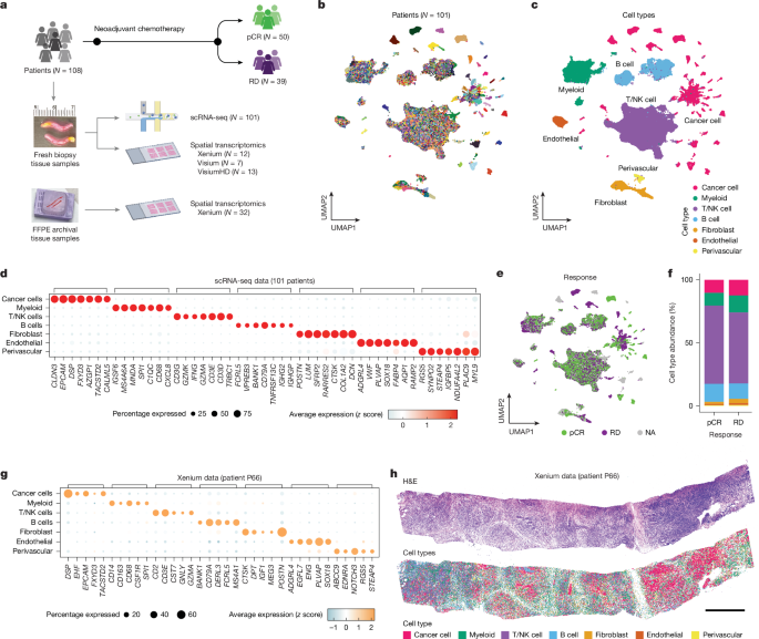
The clinical trial protocol was reviewed and approved by The University of Texas MD Anderson Cancer Center Institutional Review Board and all participants provided written informed consent (NCT02276443; MDA no. 2014-0185). All study procedures performed were in accordance with ethical standards of the Institutional Review Board and with the 1964 Helsinki declaration and its later amendments or comparable ethical standards. TNBC was defined as breast cancer that was oestrogen receptor-negative (lower than 1%) or low oestrogen receptor-positive (1% to less than 10%), progesterone receptor-negative (less than 1%) or low progesterone receptor-positive (1% to less than 10%) and HER2-negative by immunohistochemistry and fluorescence in situ hybridization. Residual cancer burden (RCB) status after chemotherapy treatment was assessed by histopathology from the resected surgical specimen⁶¹. Chemotherapy response was classified into pCR (RCB-0) or RD (RCB-I, II or III) by RCB status. A subset of patients (N = 19) with suboptimal mid-treatment response were changed to targeted therapies before surgery and had no NAC response data available. The gene-expression data from patients with TNBC without NAC response data were used for the biological analysis (for example, cell type and cell state clustering) but were excluded from the analyses comparing the response groups. For each patient, 1–4 fresh tumour breast core needle biopsies were collected and transported to the laboratory in media for cell dissociation and frozen for spatial transcriptomic experiments.

Experimental method details

scRNA-seq

The biopsies were placed in 10-cm sterile tissue culture dishes and were cut into pieces around 1 mm³, then digested in 1 ml of dissociation buffer (collagenase A (1 mg ml⁻¹ working solution, Sigma no. 11088793001) dissolved in DMEM F12/HEPES media (Gibco no. 113300) and BSA fraction V solutions (Gibco no. 15260037) mixed at a 3:1 ratio, respectively). Cell suspensions were transferred into a 1.5-ml tube and rotated in a hybridization oven for 30 min at 37 °C. The cell pellet was collected by centrifuging at 500g for 5 min and then resuspended in 1 ml of trypsin (Corning no. 25053CI) before incubating in a rotating hybridization oven at 37 °C for 5 min. Next, 2 ml of DMEM containing 10% fetal bovine serum (Sigma no. F0926) was used for trypsin neutralization. The solution was then filtered through a 70-μm strainer (Falcon no. 352350) and then centrifuged at 500g for 5 min to collect the cell pellet. To remove red blood cells, the cell pellet was nutated at room temperature for 10 min in 10 ml of 1× MACS red blood cell lysis buffer (MACS no. 130-094-183). Then 10 ml of DMEM was added to stop red blood cell lysis and then centrifuged at 500g for 5 min. The resulting pellet was washed in 1 ml of cold DMEM and then resuspended in 100 µl of cold PBS (Sigma no. D8537) + 0.04% BSA solution (Ambion no. AM2616) and filtered through a 40-μm flowmi (Bel-Art no. h13680-0040) on ice until use. Before loading, cell viability and cell counts were quantified by Trypan blue staining with the Countless II FL automated cell counter (Thermo Fisher) and their concentration was adjusted to 300–1,000 cells per microlitre. Single-cell capture, barcoding and library preparation were performed by following the 10X Genomics Single Cell Chromium 3′ protocols (V2, CG00052; V3, CG000183; V3.1, CG000204). A detailed step-by-step description of this protocol is also publicly available at Protocols.IO https://doi.org/10.17504/protocols.io.t3geqjw.

Visium spatial transcriptomics experiments

Visium spatial transcriptomics experiments were performed using the Visium Platform (10X Genomics) following the manufacturer’s protocol with a minor modification based on the recommendations in the Tissue Optimization protocol (10X protocol no. CG000238). Specifically, fresh tumour biopsies were embedded in cryogenic (cryo) moulds with optimal cutting temperature (OCT) compound (Fisher nos. NC9542860, 1437365) on dry ice and stored at −80 °C until cryo-sectioning. Next 12-μm sections were prepared on a cryomicrotome (Cryostar NX70, Thermo Scientific) with chuck and blade temperatures set at −17 °C and −15 °C, respectively. Two core sections were placed within the capture area of the Visium spatial slide (10X Genomics PN-1000184). According to the manufacturer’s tissue optimization protocol, we determined that the optimal permeabilization time for breast tissue was 12 min. Sectioned slides were fixed and stained with H&E as described by the manufacturer (10X protocol no. CG000160). Images of H&E staining were captured on the Nikon Eclipse Ti2 system following imaging guidelines (10X protocol no. CG000241). The final libraries were constructed by following the user guide (10X protocol no. CG000239) and were sequenced on the Illumina next-generation sequencing system (NovoSeq6000) using the S2-100 flow cell.

Xenium in situ RNA experiments

Fresh frozen breast core biopsy tissues were embedded in cryomolds using OCT compound (Thermo Fisher Scientific no. 1437365) over dry ice and cryo-sectioned at 12 μm using a cryomicrotome (Leica, CM1950). Sections were placed within the capture area of the Xenium slides (10X Genomics, PN3000941). Tissue fixation and permeabilization were performed according to the 10X Genomics user guide (CG000581, revision D), with a modification extending the 37 °C incubation to 3 min for breast tissue samples. FFPE tissues were sectioned at 5 μm and placed on xenium slides by the pathology laboratory. Deparaffinization and decrosslinking were performed following the 10X Genomics user guide (CG000580, revision E), with a modification extending the nuclease-free water incubation time to 1 min to remove residual eosin from previously stained tissue before embedding. Both OCT and FFPE slides were subsequently proceeded according to the Xenium prime in situ gene expression with cell segmentation staining User Guide (CG000760, revision E). A custom 100-gene panel was also designed (Supplementary Table 4) and incorporated as an add-on to the Xenium Human 5K Pan Tissue & Pathways Panel. Post-Xenium H&E staining was conducted following the manufacturer’s protocol (10X Genomics user guide CG000613 revision A).

VisiumHD spatial transcriptomics experiments

Fresh frozen breast core biopsy tissues were embedded in OCT and cryo-sectioned at 12-μm thicknesses onto Nexterion H 3D hydrogel-coated slides (SCHOTT, no. 1800434). H&E staining and imaging were performed according to the VisiumHD Fresh Frozen Tissue Preparation Handbook (10X Genomics, CG000763, revision E), with a modification extending the 37 °C incubation step to 3 min for breast tissue samples. FFPE tissues were sectioned at 5-μm thicknesses and mounted on Nexterion H 3D hydrogel-coated slides. H&E staining, imaging and decrosslinking were conducted following the VisiumHD FFPE Tissue Preparation Handbook (10X Genomics, CG000684, CG000730). Post-Xenium prime slides were processed according to Post-Xenium in Situ Applications for VisiumHD (10X Genomics, CG000709, revision D). Autofluorescence Quenching Solution was removed following the Post-Xenium Analyzer H&E Staining Protocol (10X Genomics, CG000613, steps 1.1–1.3). H&E staining and imaging were performed as described in the VisiumHD FFPE Tissue Preparation Handbook (10X Genomics, CG000684). Tissue slides were imaged using a Nikon Eclipse Ti2 microscope in accordance with the VisiumHD Spatial Applications Imaging Guidelines (10X Genomics, CG000688). Subsequent library preparation and sequencing were performed following the VisiumHD Spatial Gene Expression Reagent Kits User Guide (10X Genomics, CG000685).

Quantification and statistical analysis

Preprocessing of the scRNA-seq, Visium, VisiumHD and Xenium data

Sequencing reads of the scRNA-seq from the 10X Genomics Chromium protocol were demultiplexed using bcl2fastq (v.2.20). The scRNA-seq reads were aligned to the hg38 human genome reference using the CellRanger pipeline (v.3.1.0) with the default parameters. The Visium and VisiumHD reads were aligned to the hg38 human genome using the SpaceRanger pipeline (v.3.1.3) with the default parameters. For the VisiumHD processing, we used a bin size of 32 µm to combine features. According to the Xenium Onboard Analysis User Guide (CG000584, revision H), Xenium data and cell segmentation were generated by the xenium onboard analysis (v.3.3.0.1) using the xenium instrument software (v.3.3.0.0). The cell (or spot)-gene-expression matrix of each sample was normalized to 1 × 10⁵ and log₂-scaled using Seurat (v.5)⁶².

Identification of aneuploid cells from scRNA data

We applied CopyKAT³⁶ (v.1.0.8) to infer CNAs on the basis of gene-expression read counts from each single cell. Because our scRNA-seq data in most samples contained several cell types, we randomly picked roughly 800 cells from 1 sample from the HBCA dataset³⁴ containing all the cell types and then mixed them with each TNBC sample to run CopyKAT. With the inferred CNA profiles, we further performed quality control in each sample using the Leiden-based method developed here and the Tirosh-like method modified from a previous study³⁷. The cells from HBCA are all normal diploid cells, so they are used as the negative control to help identify any query cells with spurious CNA events.

The Leiden-based method determined aneuploidy if the query cells were not coclustered with the negative-control cells on the basis of the inferred CNAs profiles. The single-cell inferred CNAs profiles were subjected to principal component analysis (PCA). The top 30 PCA components were used to further perform dimensionality reduction to a two-dimensional space of UMAP. With the UMAP space coordinates of cells, a cell-to-cell similarity graph was built using ‘Rphenograph’ (v.0.99.1) at a granularity of using 50 nearest neighbours. On the basis of this similarity graph, the cell clusters were determined by using the function ‘leiden_find_partition’ of the ‘leidenbase’ package (v.0.1.8). To avoid under-clustering, clustering was performed stepwise with the clustering resolution, which started at 0.1 and increased by 0.1 per step. To avoid over-clustering, clustering stopped if either there were more than five clusters, or the resolution value reached two. As a result, a cell cluster was tentatively considered ‘aneuploid’ if the number and the percentage of the negative-control cells in the cluster were fewer than 10 and less than 1%, respectively.

The modified Tirosh-like method calculated the CNA score, which quantified the magnitude of genomic aberrations and the aneuploid correlation coefficient (ACC) that reflected whether a cell harboured the common CNAs profiles found in the sample. The CNA score of each cell was the square root of the sum of the squared CNA values of all genomic bins, where the CNA value was log₂-scaled copy number ratio provided by CopyKAT. It was then rescaled against a value interval with the minimum and maximum specified as the 5% and 99.5% quantile of the CNA scores of the negative-control cells, respectively. To calculate ACC, the top 1% of cells with the highest CNA score were selected to compute the average CNA profile that represented the profile of the tentative aneuploid cells. A Pearson correlation coefficient between this profile and each single-cell inferred CNAs profile was calculated to yield ACC. The 99% quantiles of the CNA scores and ACCs of the negative-control cells were used as the threshold values for filtering. As a result, a single cell was tentatively considered ‘aneuploid’ if it had higher values than these two thresholds.

Taken together, each cell was finally designated as ‘aneuploid’ if it was classified as ‘aneuploid’ by both the Leiden-based and the Tirosh-like methods. Otherwise, the cell was determined as ‘non-aneuploid’.

Default scRNA-seq preliminary analysis using Seurat

The single-cell unique molecular identifier (UMI)-count data were normalized to a total UMI count of 1 × 10⁵ and log-scaled by using ‘NormalizeData’. Z scores of genes across single-cell were calculated using ‘ScaleData’ with total UMI counts regressed out to mitigate technical artefacts in downstream clustering. The top 2,000 high variable genes were determined by ‘FindVariableFeatures’. Linear dimension reduction of PCA was performed by ‘RunPCA’ with 300 principal components. With the top 200 PCA components, a cell-to-cell similarity neighbouring matrix was constructed by ‘FindNeighbors’, which further enabled a nonlinear dimension reduction of UMAP by ‘RunUMAP’ with the default parameters (for example, n.neighbors = 30). Louvain-based clustering by ‘FindClusters’ with various resolutions from 0.5 to 3 was performed to prepare for downstream annotation.

CCA-based integration

To mitigate potential batch-effect and patient-effect on data integration, we performed anchor-based canonical correlation analysis (CCA). In brief, we assigned single cells to arbitrary batches such that these batches had a balanced number of cells to facilitate performing CCA. The top 2,000 highly variable genes were determined by ‘FindVariableFeatures’ with the ‘vst’ method in each random batch data. These random batches were integrated by using the functions ‘SelectIntegrationFeatures’, ‘FindIntegrationAnchors’ and ‘IntegrateData’ with the default parameters.

DEG analysis

The DEGs using single-cell data were identified by applying the functions ‘FindMarkers’ and ‘FindAllMarkers’ of Seurat, which uses the Wilcoxon rank-sum test and corrects P values by the Bonferroni method. The DEGs using a pseudo-bulk count matrix were identified by using the functions ‘DESeqDataSetFromMatrix ‘, ‘DESeq’ and ‘results’ of the package ‘DESeq2’⁶³ with the default testing parameters, which performed a Wald test and adjusted P values by means of the Benjamini–Hochberg procedure.

Filtering of scRNA-seq data and identifying main cell types

To remove low-quality cells, we retained cells that had at least 500 UMIs, at least 150 genes and a percentage of mitochondrial genes of less than 40%. To identify the main cell types, we computationally integrated the scRNA-seq data of all single cells of all samples using the CCA-based integration approach. Subsequently, our default scRNA-seq preliminary analysis using Seurat was performed. To identify the cell type for the resulting clusters, we identified the DEGs using ‘FindAllMarkers’ with the default parameters in a comparison of each cluster of being investigated and all the other clusters. By examining the top DEGs of each cluster, we determined the cell types on the basis of the canonical marker genes: epithelial (for example, EPCAM, KRT6A/B, KRT7, KRT19, KRT8), myeloid cells (for example, SPI1, LYZ, APOC1), T cells (for example, CD3E/D, TRBC1), NK cells (for example, GNLY, NKG7), B cells (for example, MS4A1, JCHAIN), fibroblast (for example, LUM, DCN, COL1A1/2), endothelial cells (for example, FABP4, VWF) and perivascular cells (for example, RGS5, STEAP4). Cell clusters with similar top DEGs were merged to form clusters at cell-type level.

Depending on the aneuploidy and cell-type identity, cells were separated into three groups: (1) cancer cells that were classified as aneuploid epithelial cells, (2) immune or stromal cells that were classified as non-aneuploid non-epithelial cells and (3) noisy or low-quality cells that were either aneuploid non-epithelial cells or non-aneuploid epithelial cells. Only the first two groups were kept for further processing. To remove doublets and multiplets, we enumerated each cell type and performed further clustering by applying the default Seurat clustering workflow. As previously described in ref. ³⁹, we set the highly variable genes as the canonical markers of all cell types found in the HBCA dataset to identify doublets with the cancer cells. In each cell type, any clusters expressing DEGs of other cell types were considered doublets or multiplets and were removed from analysis. Last, cell clusters with mitochondria-related and noise-related top DEGs (for example, NEAT1, MALAT1) were also removed.

Calculating the frequency of CNAs in a patient cohort

To calculate the patient frequency of a CNA event (either gain or loss) along the genome, we first determined the CNA events present in each tumour. For each tumour, we computed the median of the log-scaled copy number ratio values of each genomic bin across single cells, which resulted in the consensus CNA profile of each tumour. For each consensus CNA profile, we used the mean value of all genomic bins as the ground state copy number and the s.d. as the deviation cut-off. Then we determined that a genomic bin had a CNA event of genomic gain if its copy number was greater than the mean + s.d., whereas it had a genomic loss if the copy number was smaller than the mean − s.d. Finally, the frequency of a CNA event in a genomic bin was determined as the number of consensus profiles having that event divided by the total number of consensus profiles.

Creating pseudo-bulk RNA-seq data

To create a pseudo-bulk RNA-seq data for a given group of single cells (for example, a patient or a cell type), the UMI counts of all single cells were summed for each gene. When there were many groups, we performed variance stabilizing transformation for normalization using the ‘vst’ function in DESeq2 (ref. ⁶³) (v.1.34.0).

Performing NMF

Given a log₂-scaled normalized UMI-count matrix X_ij, where \(i\in \{1,2,\ldots ,G\}\), \(j\in \{1,2,\ldots ,N\}\), G is the number of genes and N is the number of observations (for example, cells or patients), the gene expression of each gene among observations were centred to zero and then all the negative values were modified to zero. This processed matrix was then subjected to RcppML⁶⁴ (v.0.3.7) to run non-negative matrix factorization (NMF). The parameter ‘tol’ controlling tolerance was set to 1 × 10⁻⁵ to allow sufficient iterations and achieve a high approximation. With a fixed number of factors (that is, K), NMF resulted in two matrices: W_ik showing genes-to-factors contributions and H_kj showing factors-to-observations contributions, where \(k\in \{1,2,\ldots ,K\}\). NMF was not performed when K exceeded N.

Determining marker genes of a NMF factor

Marker genes of each factor were determined on the basis of the gene-to-factor contribution matrix W_ik of NMF⁶⁴. For a factor indexed at k, genes were sorted in a decreasing order on the basis of the values in the column W_*k. Then each gene g was enumerated to be added to the set of marker genes until the specific value W_gk was no longer the maximum of the row W_g*, as previously described in ref. ⁶⁵. To accommodate genes possibly shared by several factors, we tolerated at most two more genes being added when the value W_gk was not the maximum. This procedure was later used to define marker genes for archetypes and metaprograms.

Identifying archetypes

In contrast to the conventional bulk RNA-seq that reflected signals from the intermixed cell types, we created a pseudo-bulk RNA-seq gene-expression matrix using cancer cells only for each patient and then performed NMF on all pseudo-bulk data to identify archetypes. In detail, the top 75% of genes in terms of the mean and variance of gene expressions were retained. This filtered pseudo-bulk gene-expression matrix was subjected to NMF using several numbers of factors K ranging from 2 to 10. Each factor denoted an archetype. The parameter ‘L1’ controlling sparsity of NMF results was set as 0.05. To determine the most possible number of archetypes in the dataset, we used the function ‘fviz_nbclust’ of ‘factoextra’ (v.1.0.7) to estimate the silhouette scores that compared the patient-to-patient Spearman correlation matrix of gene expressions and the archetype assignments resulting from the series of K values. Last, the resulting matrix H_kj was used to assign each patient j by its highest factor, representing the designated archetype. The gene signature of an archetype was determined as the shared genes between the marker genes of each archetype (that is, a NMF factor) and the DEGs of each archetype that showed a fold change of 2 or less and Benjamini–Hochberg-adjusted P < 0.05.

Measuring archetype specificity

For each sample, the log₂ ratio between the two top archetypes and the Tau score⁶⁶ were computed using the NMF loading matrix H for scRNA-seq data and using the overall expression levels of archetype gene signatures for Xenium data. To determine the thresholds for each metric, we used the resulting values in all samples and fitted two-component Gaussian mixture model using the ‘normalmixEM’ function in the mixtools package with default parameters. The mean of the lower component was used as the threshold. Last, if both the Tau score and log₂ ratio were below the thresholds, the archetype specificity was ‘ambiguous’ in the sample; otherwise, it was ‘dominant’.

Identifying metaprograms of cancer cells

In brief, we enumerated each sample and performed NMF on single cancer cells to identify the transcriptional programs that were heterogeneously expressed. The transcriptional programs showing similar marker genes in many samples were merged to derive metaprograms. In detail, we excluded genes having an average log₂-scaled normalized expression no greater than 0.05 and samples having fewer than 20 cancer cells. The gene-expression matrix of each sample was subjected to NMF using a series of number of factors (that is, \(K\in \{2,4,\ldots ,30\}\)). Each NMF factor represented a transcriptional program, and the marker genes of the programs were determined. Jaccard similarities between all detected programs were computed on the basis of their marker genes. A program was considered noisy and excluded if it had a Jaccard similarity less than 0.25 with its most similar program other than itself.

To find the proper clusters of the programs to form metaprograms, we repeatedly applied the following procedure of clustering, cutting, grouping, filtering and merging. Hierarchical clustering was performed on the Jaccard similarity matrix with the ‘ward.D2’ linkage method by use of the function ‘hclust’. We cut the tree into several groups of programs with a series of number of cuts (that is, \(C\in \{10,12,\ldots ,30\}\)) using the R function ‘cutree’. On the basis of the grouping result of the maximum cut C = 30, we computed the intra-group and inter-group Jaccard similarity scores. We filtered out groups having an intra-group Jaccard similarity score less than 0.1. We merged groups if they had mutual inter-group Jaccard similarity scores greater than 0.2 and were found in the same group resulting from a smaller value of cut. Each round of the procedure resulted in tentative metaprograms and was repeatedly performed until there was no further change. Last, we averaged the gene-to-factor contribution values of the NMF factors assigned to each metaprogram to make the gene-to-metaprogram contribution matrix, which was used to determine the marker genes of each metaprogram (that is, a NMF factor). Metaprograms characterized by genes associated with technical noise were excluded.

Testing the association of archetype and response

We first built the contingency table of the archetype assignments and NAC responses of the patients. Then a chi-squared test was performed using the R function ‘chisq.test’, which provided a chi-squared test statistic, degrees of freedom and a P value to evaluate significance. This test also provided the Pearson residual showing the direction of association.

CNA inference in Visium data

To find the spatial transcriptomic spots having a high abundance of cancer cells in each sample, we performed the ‘Tirosh-based’ approach modified from previous work in ref. ³⁷. In each sample, we performed CopyKAT³⁶ resulting in a CNA profile for each spot. The CNA profiles of all spots were averaged to represent the reference CNA profile of the malignant cell population. For each spot, the squared CNA values of all genomic bins were averaged to represent the aberration score. A Pearson correlation between the CNA profile of a spot and the reference CNA profile was calculated to estimate whether the spot had the common CNA events detected in the sample. Using the inferred CNA profiles of all spots, we then ran the functions ‘findSuggestedK’ and ‘findClusters’ of the package Copykit⁶⁷ to determine spot clusters harbouring similar CNA profiles. The cluster of spots with an average aberration score >0.005, an average correlation >0.3 and the known CNA events (for example, chromosome 8 gain) were classified as ‘abnormal’: otherwise, they were ‘normal’. Furthermore, depending on the average aberration score, the cancer-cell abundance of a ‘abnormal’ spot cluster was further classified as ‘high’ if it was greater than 0.045, ‘medium’ if it was in the range of 0.02–0.045 or ‘low’ if it was less than 0.02.

Identifying cell types and cell states in Xenium data

Identification of cell types and cell states used the Label Transfer approach from Seurat⁶², which integrated a reference scRNA-seq data with a query Xenium data and projected the cell identities from the scRNA data to the Xenium data. First, we created a reference scRNA-seq data by randomly down-sampling at most 1,000 cells for each cancer-cell metaprogram and TME cell state and selecting genes in the Xenium gene panel. To improve computational robustness, we performed ‘label transfer’ using a tenfold cross validation approach. We split the genes evenly into ten subsets, such that each subset maintained the same statistical distribution of gene expression as the whole gene set. Then label transfer was performed consecutively ten times with nine gene subsets used each time. Last, the consensus transferred label was used as the cell identity for each cell. In detail, we performed label transfer for each Xenium sample to determine cell types while we enumerated each cell type of the immune and stromal cell types to integrate all Xenium data to perform label transfer, which resulted in cell states. As doublets or low-quality cells did not receive the same votes for cell identities among the ten label transfer results, we required a cell to have the same transferred cell type in all the ten votes. The threshold of votes for a transferred cell state was the maximum votes, such that the total probe count, the detected gene count and the label transfer probability of cells were no longer significantly different from the cells with ten votes (Wilcoxon test, Benjamini–Hochberg-adjusted P < 0.05). If this vote threshold was less than five, it was manually designated as five. Doublets or low-quality cells were removed from this analysis.

Identifying cancer-cell bins in VisiumHD data

VisiumHD with a bin size of 32 µm was used to increase gene counts for cells. The bins with total UMI counts fewer than 10 and a gene number fewer than 30 were removed from analysis. VisiumHD data were subject to the same default scRNA-seq preliminary analysis using Seurat. The aneuploid bins were identified using the same pipeline of scRNA-seq aneuploid cell identification. Cell types of bins were identified by the Robust Cell Type Decomposition method in the package spacexr⁶⁸ (v.2.2.1). As the reference data to run Robust Cell Type Decomposition, we first leveraged the HBCA scRNA-seq data and then used the TNBC scRNA-seq data from this study. The bins that were ‘aneuploid’ and were predicted as ‘epithelial cells’ and ‘cancer cells’ were finally designated as the cancer-cell bins.

Gene signature levels in spatial transcriptomics

We used AUCell⁶⁹ (v.1.16.0) to quantify the overall expression level of a gene signature (for example, archetypes) in the spatial transcriptomics data. In brief, we used the function ‘AUCell_buildRankings’ with the default parameters to build the gene-expression ranking matrix of all genes across all spots. We applied the function ‘AUCell_calcAUC’ and specified the parameter ‘aucMaxRank’ to use the top 20% of the genes in the ranking matrix, which resulted in the ‘AUCell value’ estimating enrichment level of a gene signature in spots.

Calculating module scores of a metaprogram in single cancer cells

For each metaprogram, module scores of single cells were computed using the expression of marker genes while randomly selecting genes with comparable expression levels as the control³⁷. Specifically, we applied the function ‘AddModuleScore’ of Seurat⁶² on all cancer cells from all samples to calculate the module scores.

Assigning cell cycle phase for single cells

We applied the function ‘CellCycleScoring’ of Seurat with the cell cycle phase-specific genes provided by Seurat to all the cancer cells to assign the cell cycling phase.

Integrating TME of TNBC and the normal breast tissues

We randomly selected the scRNA-seq data of 50 disease-free individuals from the HBCA dataset³⁴. For each non-cancer cell type (that is, myeloid cells, T/NK cells, B cells, fibroblast, endothelial cells and perivascular cells), we used CCA-based integration approach to integrate the single cells from patients with TNBC and normal breast tissue data from HBCA.

Immune and stromal cell states in scRNA-seq data

For the immune (myeloid, T/NK and B cells) and stromal (fibroblast, endothelial and perivascular cells) cell compartments, we performed further subclustering for each cell type using the following procedure. Subclustering was performed by using the function ‘FindClusters’ with a series of clustering resolution ranging from 0.5 to 3. The DEGs of clusters were identified by using the function ‘FindAllMarkers’. Clusters showing similar DEGs were merged to avoid over-clustering. We also used the package ‘clustree’⁷⁰ (v.0.4.4) and referred to the results of integrating with HBCA to guide choosing the proper resolution and merging cell clusters. Cell subclusters expressing canonical marker genes from other lineages were considered doublets and removed from analysis.

Single-cell UMAP visualization of cells in scRNA-seq data

To facilitate single-cell UMAP visualization of all cells, all cancer cells, all immune cells or all stromal cells, we applied the default single-cell analysis workflow with the following adjustments of parameters. For all cells, all cancer cells and all immune cells, we simply merged the single-cell data instead of applying CCA-based integration. For all stromal cells, we used the integrated data. Then we re-identified 5,000 high variable genes and reperformed PCA with 500 components. The top 300 PCA components were used. Finally, to regenerate the UMAPs for all cells and all cancer cells, we did not adjust parameters of ‘RunUMAP’. We changed the parameters to n.neighbors = 20, min.dist = 1 and spread = 0.75 for all immune cells, and changed to min.dist = 3 and spread = 1.5 for all stromal cells.

Cell frequency of the metaprograms and TME cell states

The cell frequency of a metaprogram in a sample was calculated as the ratio between the number of cancer cells having a module score no smaller than 0.1 and the total number of cancer cells. In the sample without cancer cells, the cellular frequencies of metaprograms were assigned as ‘not detected’ (that is, the ‘NA’ value) instead of 0. The cell frequency of a TME cell state in a sample was computed as the fraction of the cell state in the corresponding cell type. This fraction was also designated as not detected if the corresponding cell type was not found in the sample. This calculation procedure was applied to scRNA-seq and Xenium data. Comparison of cell frequencies between two groups was subject to the Wilcoxon signed-rank test providing exact P values.

Co-occurrence of cancer cells and TME cells

The co-occurrence network was based on Spearman correlation coefficients (SCCs) of TME cell states and cancer-cell metaprograms using their cell frequencies among samples. We used the R function ‘cor’ with the parameter ‘use’ specified as ‘pairwise.complete.obs’ to compute SCCs and statistical significance. We then used the package ‘igraph’ (v.1.5.0.1) to convert the SCC matrix to an undirected weighted network by considering TME cell states and metaprograms as nodes and SCC scores as edge widths. Only correlations with P < 0.05 were kept for further analysis and visualization.

Determining ecotypes of cancer metaprograms and TME cell states

On the basis of the co-occurrence network, we performed community detection to determine the subnetworks to define the ecotypes. We first filtered out all edges having a negative SCC score. To find a proper clustering resolution to apply the function ‘cluster_louvain’ of ‘igraph’, we evaluated the number of ecotypes and the median size of ecotypes that each was a function of clustering resolution values ranging from 0.01 to 10. As the clustering resolution increased, the number of ecotypes increased and the median size of ecotypes decreased. We determined that the optimal clustering resolution value was where the two functions crossed. To alleviate the computational stochasticity of ‘cluster_louvain’, we performed clustering 1,000 times using the optimal clustering resolution value and built an instance matrix recording the number of times that any two nodes were clustered into the same ecotype. Finally, we applied the function ‘infomap.community’ of ‘igraph’ on this instance matrix to determine the communities that defined the ecotypes.

Visualizing the co-occurrence network

Edges with a SCC score less than 0.2 were considered spurious and were filtered out. We then heuristically changed the parameter ‘weights’ of the igraph’s function ‘layout_with_fr’ to get a graph layout to visually separate the ecotypes, while the original SCCs between any two nodes were reserved. Specifically, if an edge connected two nodes that were assigned to the same ecotype, the ‘weights’ parameter was set as 18; otherwise, it was 1. This layout was used for all graph visualizations of the co-occurrence network.

Comparing the co-occurrence network across patient categories

To facilitate comparing the co-occurrence network across patient categories (for example, pCR and RD), we computed and visualized the relative copresence (RCOP) scores among the TME cell states and the cancer metaprograms for each patient category. In detail, using the cell frequency matrix F_ij where i denoted the TME cell states and the cancer metaprograms and j denoted the patients, we calculated a z-score for each row to yield a relative cell frequency matrix Z_ij. Then for each patient category, we applied the following procedure to compute a category specific RCOP score matrix. The matrix Z_ij was subset by using the patients assigned to the specific category. The row averages of this subset matrix were calculated to yield a vector z_i. To calculate the RCOP score between a pair of TME cell states and cancer metaprograms that were indexed at a and b, we computed the geometric average \({{\rm{e}}}^{[{\rm{ln}}[A]+{\rm{ln}}[B]]/2}\), where A = z_a and B = z_b. RCOP was assigned zero if either A or B was negative. Last, we obtained a RCOP score matrix for each specific patient category, which was visualized on the graph of the co-occurrence network. To quantify the similarity between the graphs of two patient categories, we computed the Jaccard similarity of two graphs on the basis of their edges with a non-zero RCOP score.

Ligand–receptor analysis

Ligand–receptor analysis was performed using the CellChat package⁷¹. For each cancer-cell metaprogram and TME cell state, we randomly down-sampled to about 20% of the cells. We then performed the default CellChat workflow using the functions ‘identifyOverExpressedGenes’, ‘identifyOverExpressedInteractions’, ‘computeCommunProb’, ‘computeCommunProbPathway’ and ‘aggregateNet’. We then used the function ‘netAnalysis_contribution_allLR’ to obtain the probabilities of all ligand–receptor pairs to compute the intra-ecotype and inter-ecotype signals, which were used for the downstream visualization.

Spatial niche analysis in Xenium data

Spatial niches were identified on the basis of the cell composition within the regions surrounding single cells. In detail, we enumerated the Xenium data of each patient and computed the percentages of all cancer-cell metaprograms and TME cell states in the regions having a radius of 30 µm with single cells as the centres. Each cancer cell was labelled as the highest metaprogram with a module score greater than 0.1. This step generated a new single-cell data matrix representing the local cell composition of each cell in each sample. Then we clustered each cell composition matrix to identify niches in each sample. To speed up this clustering step, we applied the ‘SketchData’ function of the Seurat package⁶² to run the clustering using ‘FindNeighbors’ on 2 × 10⁵ cells in each patient and applied the ‘ProjectData’ function to provide the clusters of all cells in the sample. To avoid over-clustering, we computed the average cell percentages of these clusters that were subjected to the ConsensusClusterPlus package⁷² to merge similar clusters. Last, after we computed the average cell percentages for these robust clusters in each patient, we used all these clusters found in all patients to run clustering using the ConsensusClusterPlus package, which resulted in the spatial niches that were present in several samples. Each cell was assigned to a spatial niche. The average cell abundance across spatial niches was used for biological annotation and visualization. In addition, we applied the function ‘scoloc’ of the package CellTrek (v.0.0.94)⁷³ with the parameter ‘use_method’ set to ‘DT’ to compute the spatial colocalization odds ratio matrix among cell states that were averaged on the basis of the niches to run hierarchical clustering and determine the spatial relationship between niches.

Selecting patients and treatment arms in public cohort datasets

To obtain validation datasets that were comparable to this study, we selected the pretreatment bulk sequencing-based gene-expression datasets of patients with TNBC from four public clinical trials including SCAN-B⁵⁶ and I-SPY2⁴⁵, as well as BrighTNess⁴⁴ in which patients received neoadjuvant therapy and METABRIC⁴⁰ in which patients received adjuvant therapy. First, we subset the patients who were either labelled as TNBC or were negative for the expression of endoplasmic reticulum, PR and HER2 as recorded in the original clinical metadata. For METABRIC, all the treatment arms containing chemotherapy were used in all the analysis. For SCAN-B, only the chemotherapy arm was used in all the analysis. For I-SPY2 and BrighTNess, all the treatment arms containing chemotherapy were used for the application of the 13-gene model.

Predicting the archetypes in external TNBC cohort data

The bulk RNA-seq data matrix of an external cohort was first subjected to same rescaling step of the section ‘Performing NMF’. This rescaled matrix was then combined with the NMF input data matrix of our samples, which was an internal control. We used this combined matrix to run the same NMF procedure using the RcppML package with a rank of 4. By leveraging the archetype designation of our TNBC data, we renamed each resulting cluster to the archetype showing the highest matches. Accuracy of the prediction in each external cohort was assessed by the percentage of the predicted archetypes that matched the established archetypes in our TNBC samples.

Survival analysis using the Cox proportional-hazards model

To assess how numeric variables (for example, age, module score of a gene signature and risk score predicted by a model) were associated with overall survival of patients in a cohort, we applied the Cox proportional-hazards model to the variables of interest and the overall survival data. To compute a gene signature, the overall expressions in patients were computed using the function ‘gsva’ of the package ‘GSVA’⁷⁴ (v.1.42) with the parameter ‘method’ set as ‘ssgsea’, and then the z-score was computed. We used the function ‘coxph’ of the package ‘survival’⁷⁵ (v.3.3) to construct the Cox proportional-hazards model. The hazard ratios and P values of the Wald test were extracted from the modelling result and visualized using the function ‘ggforest’ in the package ‘survminer’ (v.0.4.9).

Building the cell-state-based classifier to predict NAC response

Considering the TME cell states and cancer-cell metaprograms as features, we excluded features detected in no more than ten samples. Samples without response data were excluded from this analysis. We randomly split samples into 70% for training and 30% for testing. Because the number of features was greater than the number of training samples, we performed a preliminary feature selection by univariate logistic regression and retained the features with a P value less than 0.1. With these informative features, we used the package ‘caret’⁷⁶ (v.6.0-90) to train the following three models: logistic regression, linear discriminant analysis and random forest. During the training, the fivefold cross validation was repeated five times. The performance of each model was evaluated on the testing dataset and visualized by using the ‘pROC’ package⁷⁷ (v.1.18). The feature importance values were computed by running caret’s function ‘varImp’ on each model.

Building the gene-based classifier to predict NAC response

We started with a pool of candidate genes that were associated with chemotherapy response using: (1) the marker genes of the cancer metaprograms and archetypes, (2) the DEGs across the TME cell states and the cancer cells labelled by the most dominant metaprogram and (3) the DEGs of the TME cell states and the cancer cells labelled by the most dominant metaprogram in a comparison of pCR and RD. Using the pseudo-bulk RNA-seq data derived from all cells, we enumerated each gene and applied univariate logistic regression to find the genes significantly predicting chemotherapy response (P < 0.01). As a result, 13 genes were identified and then were used to build a multivariate logistic regression model to yield a risk score for predicting the likelihood of a patient having RD.

The gene-based classifier and overall survival

The METABRIC⁴⁰ and SCAN-B⁵⁶ cohorts were used for this survival analysis. For each gene, we first rescaled its expressions among the patients in the external cohort into the value range of the expressions in our pseudo-bulk data, to mitigate possible batch effects. Then patients were stratified into high-risk and low-risk on the basis of the mean of the predicted risk scores. We used the function ‘survfit’ of the package ‘survival’⁷⁵ (v.3.3) to compare the difference of the overall survival curves between the two groups. The P value of the LogRank test was extracted by the function ‘surv_pvalue’. The Kaplan–Meier plot was visualized by ‘ggsurvplot’ of the package ‘survminer’ (v.0.4.9).

Gene signatures of the ‘Vanderbilt’ expression subtypes

Because the original study of ‘Vanderbilt’ subtypes⁹ did not directly provide the gene signatures for each subtype, we downloaded and processed their DEG results. In detail, we retained the DEGs that were labelled as ‘upregulated’ in each subtype and had an adjusted P value of less than 0.05. The original gene alias names were converted to the updated gene symbols using the function ‘alias2Symbol’ of limma⁷⁸ (v.3.50.3). The resulting gene signatures are available at Zenodo (https://doi.org/10.5281/zenodo.10846115)⁷⁹.

Reporting summary

Further information on research design is available in the Nature Portfolio Reporting Summary linked to this article.